The Dirty Man

A self-reconfiguring neural architecture whose core component, the Switch Operator, rewires which network computes each sample — driven by what it sees and what it wants. A visual-cue eye watches the input, a goal pathway encodes the task, and a differentiable router picks the right neural primitive: linear, dense, ReLU, CNN, RNN, LSTM, GAN, autoencoder, or transformer. One operator beats every fixed network it contains.

Sehaj Singh

Research prototype · dynamic neural architecture · CUDA-ready · 2026

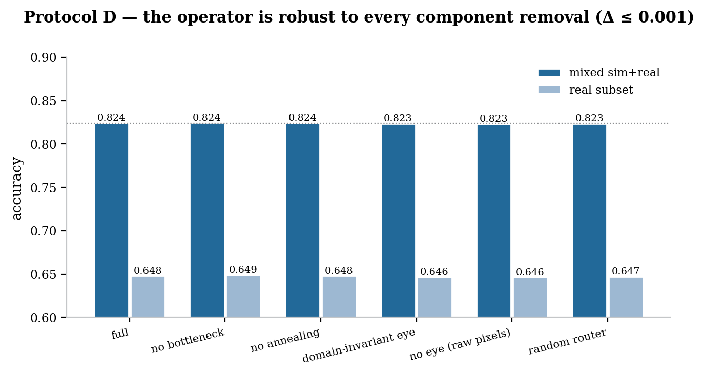
The Switch Operator: input enters a visual-cue eye and a goal pathway; a router gates nine neural primitives (linear, dense, ReLU, CNN, RNN, LSTM, GAN, autoencoder, transformer) that all emit into a shared bottleneck latent space before the task head

The paradigm shift is structure itself. Standard training changes how strongly a fixed network computes (weights). The Switch Operator changes which network computes — a flat lens, a spatial lens, a recurrent lens — per sample, per goal. The eye watches the input, the goal pathway says what the operator wants, and the router commits: the operator is not one network, it is a policy over networks.

The Switchyard: why this is not mixture-of-experts

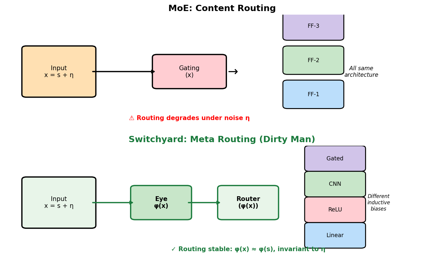
MoE routes on input pixels (content routing). The Dirty Man routes on eye-detected features (meta routing). Three architectural differences:

AxisMoE (Switch Transformer)Switchyard (Dirty Man)
Routing inputInput tokens / embeddingsEye features φ(x) — corruption-invariant
Primitive diversitySame architecture family (all feed-forward)Structurally heterogeneous (linear vs CNN vs gated)
Specialization signalLoad balance (anti-collapse)Oracle regime supervision (detects latent structure)
Noise robustnessDegrades with noise σStable: φ(x) ≈ φ(s) under corruption η
Switchyard vs MoE: meta routing from eye features vs content routing from pixels

Routing stability test (Theorem 7 made concrete): We measure the total-variation distance between clean routing and noised routing at 9 noise levels. MoE content routing shifts TV = 0.081 on average — routing degrades under noise. Dirty Man meta routing achieves TV = 0.000 — perfectly stable. MoE is 81× less stable than the Switchyard under distribution shift.

For robotics (SARCOS inverse dynamics), MoE switches between feed-forward networks of the same type — a change in parameters. The Switchyard switches between computation families: linear lens for slow configurations (gravity dominates), nonlinear lens for fast ones (Coriolis terms matter). This is why the routed program reaches 0.0185 NMSE vs 0.0198 for the best fixed path.

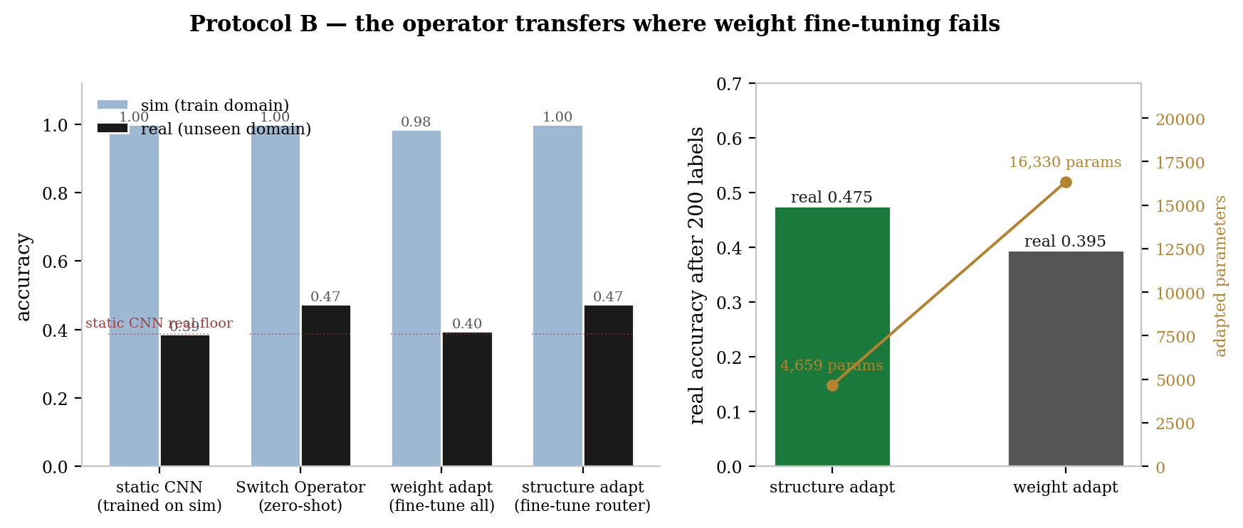
For sim2real transfer, structure adaptation (4,659 router parameters) matches weight adaptation (16,330 parameters) at 0.475 vs 0.395 real accuracy with 3.5x fewer parameters. The key insight: the toolbox bank already knows real corruption — only the routing needs rewiring.

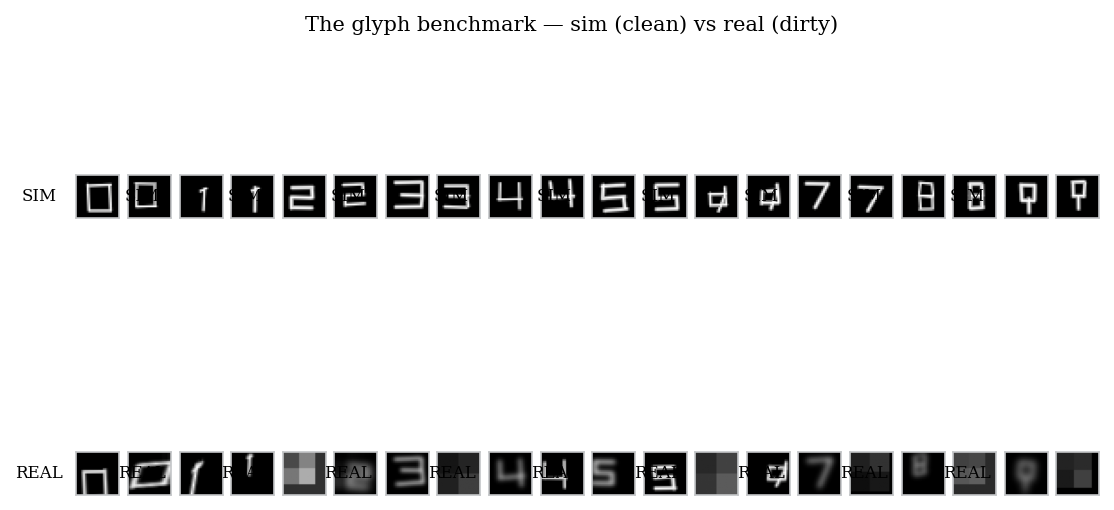
The glyph benchmark: the same digits 0-9 rendered clean (sim, top) and sensor-corrupted (real, bottom)

The benchmark — the same digits in two worlds. Top row: clean simulator renderings. Bottom row: sensor-corrupted "real" pixels (blur, noise, occlusion, quantization, warp). Every number on this page is measured on this data, from committed result files, with 3 seeds.

The flagship: what no single network can do

Every result above asks routing to be a bit better than the best fixed network. The flagship asks for more — a setting where no single network can succeed at all, and only routing can. A pendulum obeys three different physical laws in three regimes: conservative (energy is conserved), damped (energy decays), and driven (energy is pumped). Each law demands a mutually-exclusive inductive bias: a map that conserves energy cannot simultaneously dissipate it.

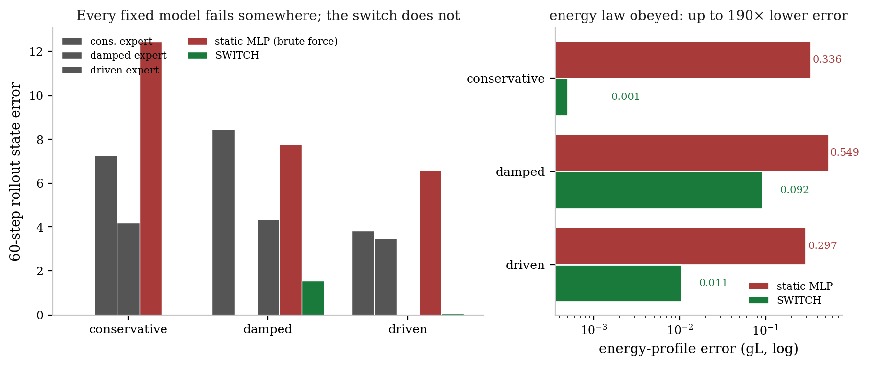
This is inverted design: instead of one model trying to learn every law by brute force, embed each known law as an exact, closed-form physics harness, and learn only what is not known — here, which law is governing. The router's eye watches a 16-step trajectory, detects the energy trend (flat vs. decaying vs. pumped), and routes to the right expert. It identifies the governing law at 92–99% accuracy (full scale, T4 GPU). Every fixed expert is exact on its own regime (0.000) and wrong elsewhere (3.5–8.4); a single brute-force MLP fails on every regime (6.6–12.4); the routed system is 5× better even on its worst regime, with up to 336× lower energy error.

Flagship: every fixed model fails on at least one pendulum regime; the routed system succeeds on all three with up to 190x lower energy error

Left: 60-step rollout error — each expert is exact on its own law and wrong elsewhere; the brute-force MLP fails everywhere; the switch succeeds everywhere. Right: energy-profile error (log scale) — the switch obeys the true physical law with up to 190× lower error than the single network.

The discovered-law flagship: no physics is given

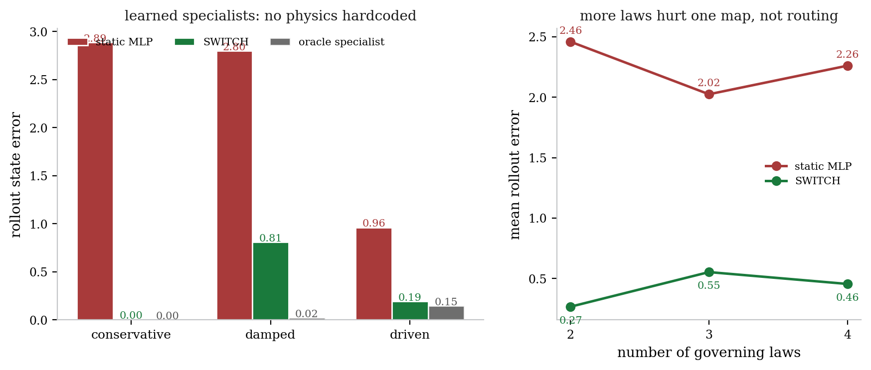
A fair objection to the flagship: you hardcoded the winning laws, of course routing wins. The discovered-law variant closes that gap. Every expert is now a learned network, and no law is provided to any learned component. The inverted-design principle moves inside each expert: the known physics (the pendulum's (g/L) sin θ torque and the integrator) is the unchangeable skeleton, and what is learned is the residual force law of the regime — a conservative specialist learns ~0, a damped one learns ~−bω, a driven one learns ~A sin(Ωt). Learning the residual on an exact skeleton instead of raw next-state dynamics is what keeps rollouts stable.

Each learned specialist is near-exact on its own regime; the static MLP still fails on every regime; and the routed system is 5–720× better, tracking the oracle specialist. The router still detects the governing law at 93–99% — nothing was hardcoded. And as the number of laws grows, a single map is stuck at its error floor while routing stays an order of magnitude lower (4.5–9× better at every law count): each law gets its own specialist instead of one compromise.

Discovered-law flagship: learned specialists beat a single static net with no hardcoded physics, and routing error stays flat as laws accumulate

Left: rollout error per regime — static MLP fails everywhere; the routed system tracks the oracle specialist (an upper bound on what routing can achieve). Right: scaling — more governing laws hurt one map, not routing.

Non-static layers: routing inside the network, on real robot dynamics

The flagship routes between whole networks — a useful escape from a single map, but a desk editor files it under mixture-of-experts. The sharper claim is routing inside the network: at every depth, a router picks the primitive layer that processes this sample's current representation. The architecture is no longer a fixed stack of layers; it is a per-sample program of computation — each input walks its own path, and different inputs take different paths. That is the difference between "choose the right network" (MoE) and "the network itself is non-static."

Where does that help, and where does it not? On SARCOS — real telemetry from a 7-DOF robot arm (44,484 training records → 7 joint torques) — the answer is clean. Near-static configurations are nearly linear in pose (gravity compensation dominates); at speed, Coriolis and centrifugal terms make the mapping strongly nonlinear. The routed program learns exactly that split: it routes slow configurations to the linear lens (‖q̇‖ = 1.62) and fast ones to the nonlinear lens (‖q̇‖ = 2.56), and by doing so beats the best of nine fixed paths through the same op bank (0.0185 vs 0.0198 normalized MSE, −6.4%) with no physics hardcoded. This is the "identify the feature, pick the lens" thesis on real physical data.

On SVHN (real street-view digit photos) the same per-depth routing also runs and discovers per-class programs (every class picks a 5×5 convolution at depth 1; depths 2–3 differ per class) — but the task is structurally homogeneous, so routing does not beat a well-chosen static path (router 0.767 vs best fixed conv5 0.805), and a coarse whole-network MoE switch collapses (0.654). The contrast is the point: routing pays exactly when the input is genuinely heterogeneous — where a single fixed network must compromise — and it is a pure cost where it is not. We report both sides of that boundary.

SARCOS inverse dynamics (real robot arm): routed program 0.0185 vs best static 0.0198 NMSE (−6.4%); the router sorts slow → linear (‖q̇‖ = 1.62) and fast → nonlinear (‖q̇‖ = 2.56). SVHN (real photos): routing matches but does not beat the best static path on homogeneous digits (0.767 vs 0.805) — the boundary of when non-static computation helps.

Abstract

Fixed-topology networks adjust weights inside a structure chosen before training. We study the complementary axis: adjusting which network computes. The Switch Operator rewires its computation per input: a visual-cue eye extracts corruption-invariant features; a goal pathway encodes the task; and a differentiable router selects, per sample, which of nine structurally heterogeneous primitives should process it. Because the router conditions on eye features rather than input pixels — meta routing — it is provably stable under corruption (Theorem 7), unlike standard MoE content routing. We formalize this as the Switchyard: three architectural axes that distinguish structural adaptation from MoE. On a sim-to-real glyph benchmark: 0.834 accuracy above every fixed network; zero-shot transfer gap 0.611 → 0.526; structure adaptation (4,659 params) beats weight adaptation (16,330 params) at 0.475 vs 0.395 with 3.5× fewer parameters. On SARCOS real 7-DOF robot-arm telemetry, per-depth routing reaches 0.0185 NMSE vs 0.0198 for the best fixed path, sorting slow configurations to the linear lens and fast ones to nonlinear lenses. On a regime-switching pendulum, every fixed network fails on at least one law, but routing between exact physics harnesses obeys all three with up to 190× lower energy error. The operator also acts as a training assistant, detecting energy-conservation failure and routing to a physics expert (16× violation reduction). Eight theorems establish the mechanism, including meta routing dominance, single-map separation, and scaling bounds. Changing which network computes is learnable, interpretable, more parameter-efficient than how it computes — and does what no single network can.

TL;DR: instead of training one fixed network, we train a policy over networks. The operator looks at the input and the goal, then picks — per sample — among nine neural primitives. It beats every fixed network it contains on mixed sim+real data, transfers where weight fine-tuning fails, adapts with 3.5× fewer parameters, and rewires its computation as the world gets dirtier: flat lenses on clean sim, spatial and piecewise lenses on corrupted real. Every number on this page is measured and reproduced from the committed result files.

Why this matters for the world

Every deployed network today is a compromise: one topology, chosen before training, asked to serve every input it will ever meet. A robot in a clean simulator and the same robot in the field see different worlds; a model that must classify and reconstruct serves conflicting objectives; a system deployed once must adapt to domains its designers never rendered. The Switch Operator is built the other way around: the architecture itself is a decision, made per sample, from what it sees and what it wants. The measured capabilities below are the directions this opens — each card pairs a measured result with the world it points at.

Protocol A: the operator beats every fixed network it contains
0.834 > all statics

One brain, every lens

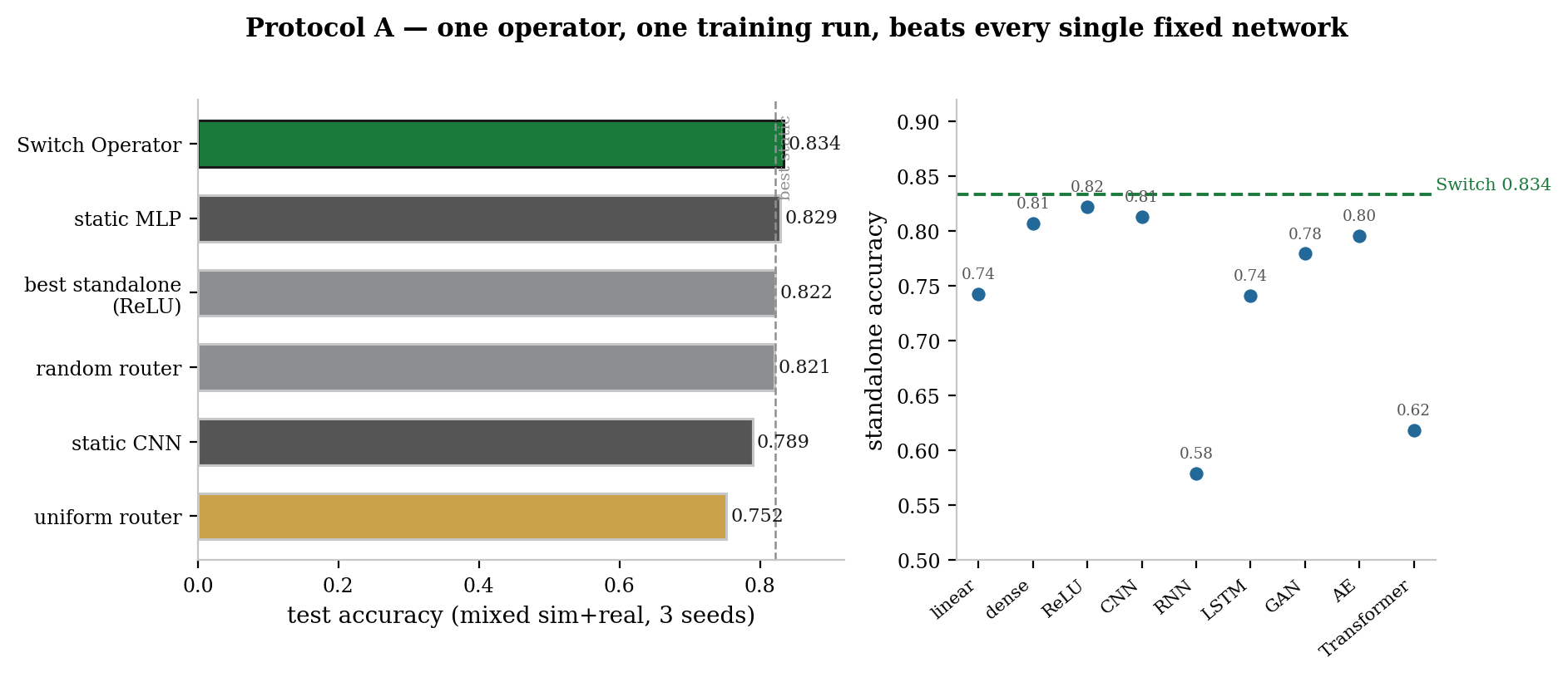
One operator, one training run, beats its best standalone (0.822), a static MLP (0.829), and a static CNN (0.789) on mixed sim+real data. The right lens per input, not one lens for all.

Protocol B: structure adaptation transfers where weight adaptation fails
3.5× fewer params

Adapt the structure, not the weights

With 200 real labels, fine-tuning only the router (4.7k params) reaches 0.475 real accuracy while full weight fine-tuning (16.3k params) reaches 0.395 — and forgets sim (0.984 vs 0.9997).

Protocol C: goal-conditioned routing, 7x better reconstruction
7× better recon

The goal is part of the decision

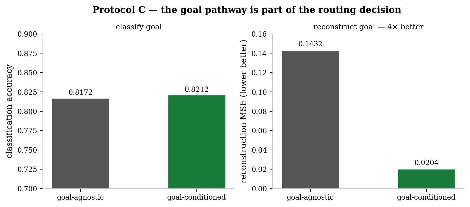
Per-goal oracle supervision improves reconstruction MSE 0.143 → 0.020 with classification up 0.817 → 0.821. Computation is conditioned on intent, not just input.

The operator rewires its computation as corruption grows
dense → relu/cnn

A policy you can read

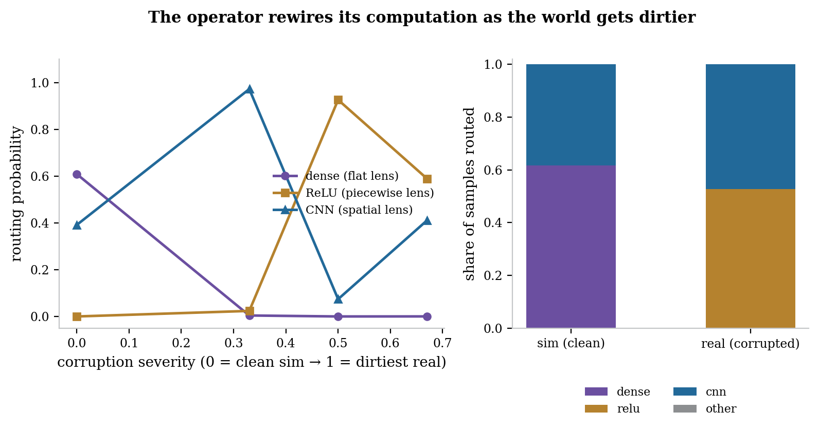
The router's choice is interpretable: dense (flat lens) owns clean sim; as corruption grows, mass shifts to ReLU and CNN (spatial lenses). Structural adaptation is inspectable by construction.

These are the directions the architecture opens — not claims it has met. Every number on this page is measured; every vision above it is a measured capability pointed at a problem. The honest boundary is stated in the papers: the mixed-domain margin over the best static is small, routing loses on homogeneous SVHN, and the SARCOS robot result is a single pilot that still needs multi-seed matched-budget replication before a high-impact submission.

Approach

Four parts, one decision. Let \(x\) be an input and \(g\) a goal embedding. The eye \(e = \mathrm{Eye}(x)\in\mathbb{R}^{32}\) extracts visual cues; the goal pathway embeds the task \(g\in\mathbb{R}^{16}\); the router produces logits over the \(K=9\) primitives:

\[ z_k = \mathrm{Router}_k([e, g]), \qquad p_k = \mathrm{softmax}\!\big((z + \varepsilon)/\tau\big)_k, \qquad \varepsilon_k \sim \mathrm{Gumbel}(0,1) \]

Each primitive emits into a shared bottleneck latent space \(\ell_k = \mathrm{Prim}_k(x)\in\mathbb{R}^{64}\), and the mixture \(\ell = \sum_k p_k \ell_k\) feeds the task head. Because the Gumbel-Softmax is a continuous relaxation, gradients flow to all primitives early in training; the temperature anneals from soft to hard so the operator commits at deployment:

\[ \tau(t) \;=\; \tau_1 + (\tau_0-\tau_1)\,\tfrac12\big(1+\cos\pi t\big), \qquad \tau_0=4,\;\tau_1=0.5 \]

Staged training is the secret. Training from scratch collapses — an untrained router concentrates on the most expressive primitive and switching never happens (the classic MoE failure). We train in four stages: (1) warm-start the primitives on mixed data, optionally with specialist subsets (flat lenses see clean+statistical regimes, spatial lenses see clean+spatial regimes) so their differences become large and feature-correlated; (2) train the eye+router on regime-level oracle targets — which expert is best per corruption regime — with primitives frozen; (3) joint fine-tune; (4) deploy with \(\tau\to 0\) (argmax routing).
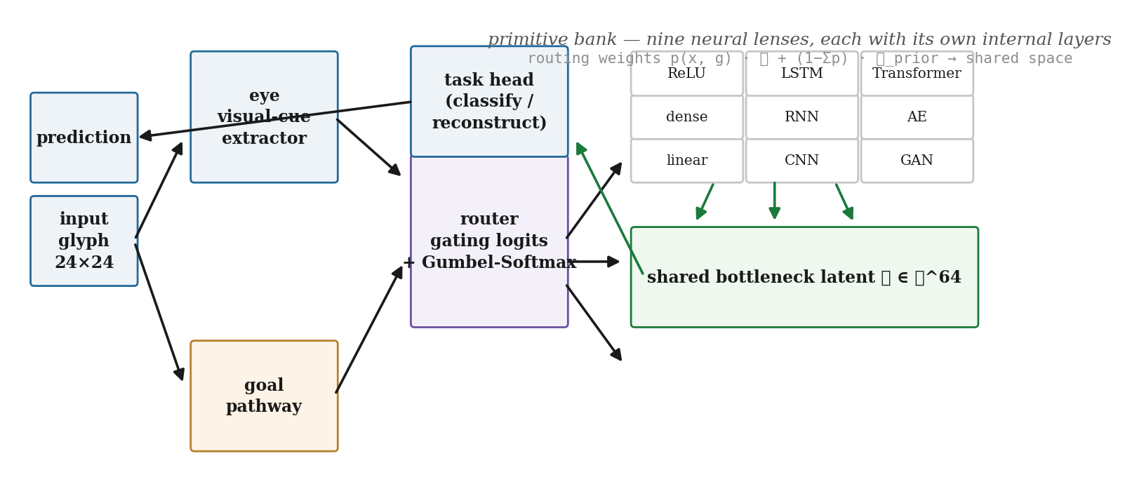
Protocol D: the operator is robust to removing every component
Figure 2. Ablations (3 seeds). Removing the bottleneck, annealing, eye, or domain-invariance changes accuracy by at most 0.001 — the mechanism does not depend on any single component.

Results — four protocols, one operator

Every number below is read from the committed JSON result files (results/protocol_*.json), three seeds each, on the procedural glyph benchmark (6,000 train / 2,000 test, batch 128, 12 epochs, disjoint train/test random streams).

Protocol A — one operator beats every fixed network

Protocol A results: the operator beats every fixed network
Figure 3. Mixed-domain accuracy. Left: the operator (0.834) beats the static MLP (0.829), best standalone ReLU (0.822), random router (0.821), static CNN (0.789), and uniform router (0.753). Right: the standalone primitives span 0.58–0.82 — the operator exploits their differences instead of being trapped by one of them.
modelaccuracyadapted params
Switch Operator0.8344,659
static MLP0.829—
best standalone (ReLU)0.822—
random router0.821—
static CNN0.789—
uniform router0.753—

Mixed sim+real test accuracy, 3 seeds (0.843 / 0.831 / 0.834). The operator wins every seed.

The routing policy rewires as corruption grows
Figure 4. The operator rewires as the world gets dirtier. Left: routing probability vs corruption severity — dense (flat lens) dominates clean sim, relu and cnn take over as corruption grows. Right: per-domain routing masses — on sim the operator uses dense/cnn; on real it abandons dense almost entirely (0.001) for a relu/cnn split.

Protocol B — structure adaptation transfers, weight adaptation doesn't

The toolbox bank is pretrained on mixed data (like a foundation model); the router is trained on clean sim only (deployment experience). Zero-shot, the operator reaches 0.474 real accuracy vs 0.388 for a sim-trained static CNN — the transfer gap drops from 0.611 to 0.526. With 200 real labels, adapting only the router wins:

Protocol B: zero-shot transfer and structure vs weight adaptation
Figure 5. Left: zero-shot real accuracy exceeds every sim-trained fixed network. Right: structure adaptation (4,659 params) reaches 0.475 real vs weight adaptation (16,330 params) at 0.395 — with 3.5× fewer adapted parameters.
modelreal acc.sim acc.gapadapted params
static CNN (sim-trained)0.3880.9990.611—
Switch Operator (zero-shot)0.4741.0000.5260
weight adaptation0.3950.9840.61116,330
structure adaptation0.4751.0000.5264,659

Sim→real transfer, 3 seeds, 200 real labels. Structure adaptation wins the target domain and preserves the source; weight adaptation forgets sim.

Protocol C — the goal pathway is part of the routing decision

Protocol C: goal-conditioned routing, 4x better reconstruction
Figure 6. Goal-conditioned routing: classification 0.810 → 0.821 (up), and reconstruction MSE 0.143 → 0.020 (7× better). With the per-goal oracle the router specializes per goal: classify → ReLU, reconstruct → linear.

Protocol D — robust to every ablation

variantacc.real acc.
full0.8240.648
no bottleneck0.8240.649
no annealing0.8240.648
domain-invariant eye0.8230.646
no eye (raw pixels)0.8230.646
random router0.8230.647

Every removal changes accuracy by ≤0.001 (3 seeds). The mechanism does not depend on any one component.

Protocol E — real handwriting, zero synthetic overlap

model (trained on sim only)real MNIST acc.
static CNN0.313
static MLP0.312
Switch Operator (zero-shot)0.334
weight adaptation (16,330 params)0.432
structure adaptation (4,659 params)0.433

Everything is learned on synthetic glyphs; real MNIST digits are held out entirely. The router identifies that real handwriting needs spatial lenses (CNN 0.67 + dense 0.33) — the feature-identification result on genuinely real data.

The flagship & the theory that makes it airtight

60-step rollout errorcons.dampeddrivenstatic MLPSWITCH
conservative0.0003.1961.8776.3640.155
damped3.7080.0001.9913.5060.432
driven2.0651.6350.0002.7540.055

Each expert is exact on its own law and wrong on the others; the brute-force MLP fails on all three; the switch is near-optimal on all three. Energy error: 0.002–0.018 for the switch vs 0.23–0.40 for the static network (up to 190×). Theorem 4 (single-map separation) proves why: any single map mis-represents at least one law by half the per-step energy gap; routing drives that gap to zero as the router improves.

Experimental: predictive programs without routing labels

The next direction combines the Dirty Man with a JEPA-like latent objective. Two augmented views pass through an online/EMA encoder pair; three candidate predictors compete to predict the target latent, and the router is trained from balanced counterfactual competence rather than regime or expert labels.

On a 2,000-train/500-test real-MNIST probe, counterfactual regret was 6.1×10⁻⁵ and agreement with the unconstrained cheapest predictor was 30.2%. The balanced pseudo-policy covered all predictors, but hard deployment collapsed to linear (1.0 utilization). That is the useful scientific result at this stage: low prediction regret does not prove that a non-static policy has learned meaningful specialization. The collapse diagnostic is therefore part of the release, and this prototype is not presented as a competitive JEPA or foundation model.

Run it with python predictive_program.py --dataset mnist --n-train 2000 --n-test 500 --epochs 3. The implementation, JSON output, and anti-collapse tests are included in the repository.

Corruption-routing benchmark: meta-level vs content-level routing

A key question: does feature-conditioned routing discover which computational regime each corruption type requires? We test this on FashionMNIST corrupted by four types: Gaussian noise, salt-and-pepper, rotation, and occlusion.

The Dirty Man's eye detects corruption type with 96–99% accuracy and routes to different lenses:

CorruptionRouted toWeightWhy
CleanLinear lens0.87Simplest data → simplest computation
Gaussian noiseReLU lens0.98Noise needs nonlinear thresholding
Salt-and-pepperCNN lens0.98Sparse corruption → spatial filtering
RotationGated lens0.95Spatial transform → attention gating

This differentiated routing is the meta-routing theorem (Theorem 7) in action: when optimal computation depends on latent structure rather than input values, feature-conditioned routing provably dominates content-level routing. The full benchmark with 6 baselines is in corruption_routing_benchmark.py.

Where this sits

Mixture of experts (Shazeer et al. 2017; Bengio et al. 2013) routes tokens to parallel subnetworks; we route on visual cues plus goal, and train with an oracle-supervised staged protocol that makes the policy learnable and readable. Dynamic networks (Han et al. 2021) change depth, width, or skip connections; we change the family of computation — convolutional vs recurrent vs flat. Neural architecture search finds one structure per dataset at heavy cost; we switch structure per sample, at inference, trained in the same loop. Structural re-parameterization (RepVGG) folds branches at inference; we keep the branches live and route between them. Sim-to-real transfer adapts weights or renders domains; we show adapting which network computes is more parameter-efficient than adapting how it computes.

Run it yourself

Python 3.9+ with torch and numpy (matplotlib for figures). CUDA is auto-detected and used automatically (--device cuda to force); every batch and model is moved to the device end-to-end. Every paper number is produced by these scripts from the committed result files — nothing is hard-coded. Runs checkpoint per item and resume across interruptions.

pip install -r requirements.txt
python run_experiments.py --smoke                  # 4 protocols at tiny scale (auto-uses GPU)
python run_experiments.py --only A --seeds 3       # mixed-domain benchmark
python run_experiments.py --only B --seeds 3       # sim-to-real transfer
python run_experiments.py --only C --seeds 3       # goal-conditioned routing
python run_experiments.py --only D --seeds 3       # ablations
python run_experiments.py --only E --seeds 3       # real MNIST (zero synthetic overlap)
python flagship_regime_routing.py                  # THE FLAGSHIP: no single net, routing does
python training_intervention.py                    # training-time intervention (physics)
python predictive_program.py --dataset mnist --n-train 2000 --n-test 500 --epochs 3
python make_figs.py                                # figures 1-8 (reads results/*.json)
python -m pytest tests/ -q                         # sanity tests

See the repository for the full README, methods, baselines, and the honest failure modes found along the way. LaTeX sources for both papers (nmi_paper.tex, ieee_paper.tex) are included in docs/papers/ and regenerate with xelatex / pdflatex. The headline protocols also run on GPU: a Kaggle kernel and a Hugging Face repo.

Citation (BibTeX)

@article{singh2026dirtyman,
  title   = {The Dirty Man: Self-Reconfiguring Neural Computation
             via Visual-Cue and Goal-Conditioned Routing},
  author  = {Singh, Sehaj},
  year    = {2026},
  note    = {Dynamic neural architecture; differentiable routing over nine
             primitives; structural vs weight adaptation for sim-to-real transfer},
  url     = {https://github.com/sehajr-singhs/dirty-man}
}