Morphogenetic Bi-Modal Networks

A neural network whose neurons carry angles, not just weights. Weights say how strongly; angles say where — and the two multiply into the connection. The network learns physical laws from noisy local observations with no global loss and no backpropagation, and its angles self-organize into a shape: a readable, mechanistic map of what it learned. Angles are the computation; the shape is the interpretable spectrum.

Sehaj Singh

Research prototype · gradient-free local learning · 2026

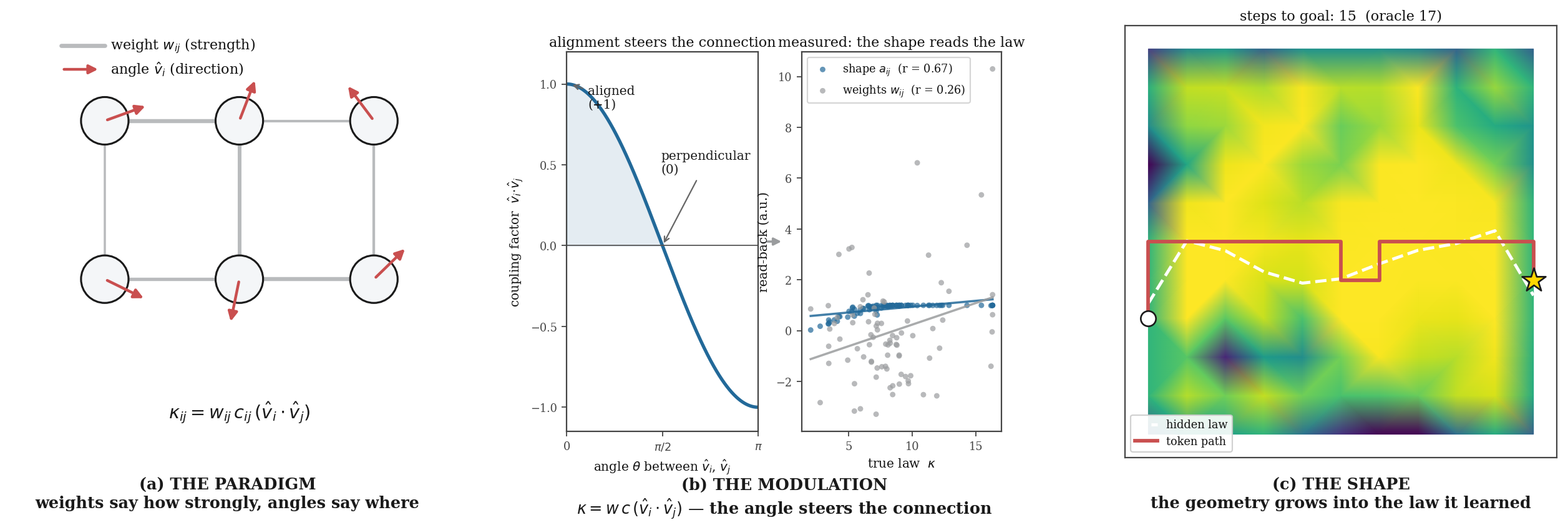
The angle paradigm in three panels: (a) two channels per neuron - scalar weights for strength and a 3D angle for direction; (b) the angle modulation kappa = w*c*(vhat_i dot vhat_j) with measured readback - the shape reads the law at r=0.67 vs r=0.26 for raw weights; (c) morphogenesis - the geometry grows into the hidden law and routes a token to the goal

The paradigm shift is the angle channel. Weights are not enough — they say how strongly but nothing about where. Every neuron in this network carries a 3D angle that multiplies the weight channel (panel a); alignment steers the connection (panel b); and the geometry that self-organizes is a readable shape — a mechanistic map of the learned law that routes real computation through the material (panel c). Angles are the computation; the shape is the interpretable spectrum.

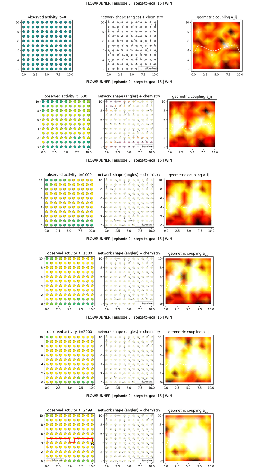
Flowrunner: the morphogenetic network plays a maze — the shape grows along the hidden corridor and a token follows it to the goal

Flowrunner — the network is shown the maze's noisy potential field, never the layout. Its streaming weak-form identifier learns the hidden law and its angle channel grows a corridor along it (dashed: the hidden truth). A token then follows the shape to the goal — from noisy observations alone, no labels, no backprop.

Abstract

We introduce a spatially embedded, gradient-free neural architecture whose computation is split across two channels: scalar weights (identified per-edge, in-stream, by a recursive least-squares loop fed by an IIR spacetime weak form that throws derivatives off noisy data and onto an analytical test function) and a 3D angle channel (a chemical-gated nematic consensus that rotates each neuron's structural vector toward its neighbors). The two multiply: \(\kappa_{ij} = w_{ij}\,c_{ij}\,(\hat{\mathbf v}_i\!\cdot\!\hat{\mathbf v}_j)\) — weights say how strongly, angles say where. The emergent shape is not decoration: it is a spatially coherent, denoised readout of the learned mechanism (r = 0.64 vs 0.35 for the raw weights), and routing through the material fails without it. On two independent real records — the 277-year sunspot series and the 78-year El Niño SST index — the same frozen streaming identifier generalizes to unseen decades at 481× and 22× lower holdout error than finite-difference identification, stays flat under 50% added measurement noise, and at 10% of the ENSO data beats a trained LSTM 5.3× at one-month forecasts while the reservoir collapses. The network scales to 104 nodes (identification improving with size, per-node cost sublinear, ~630× less memory than a reservoir), with four theorems — noise floor, contraction, monotone self-organization, and closed-loop stability — verified numerically. Angles are the computation; the shape is the interpretable spectrum.

TL;DR: we use angles now. A neural network with two compute channels — scalar weights (strength) and 3D angles (direction) — where the angles multiply the weights into the connection. It learns laws from noisy streaming observations with no backprop, its angles grow into a readable shape — a map of the law — and it plays a maze it never saw. Every number on this page is measured and reproduced from the committed result files.

Why this matters for the world

Modern deep learning is a data-center computation: training needs a global loss, a backward pass, and a GPU farm — then the trained weights are shipped to a device that can only run them, never learn. It is also a scalar computation: a weight is a number, so a network is a bag of numbers — inscrutable until someone attaches a microscope to it. This architecture is built the other way around: every neuron carries an angle, the angles are computation, and the geometry they form is the mechanism you can read. Every update is strictly local and streaming, so the same network that uses the world can learn from it, continuously, where it lives. The measured capabilities below are the directions this opens — each card pairs a measured result with the world it points at.

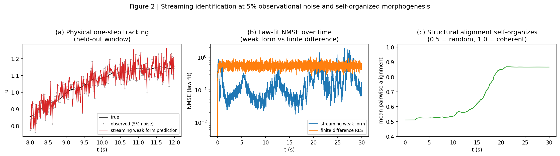
Learning curves: streaming weak form converges to 0.038 NMSE with no backprop
No backprop

Learning where it lives

No global loss, no backward pass, no label. A robot, sensor, or phone could learn from its own stream of experience — forever, on-device, in real time — instead of shipping data to a cluster and weights back.

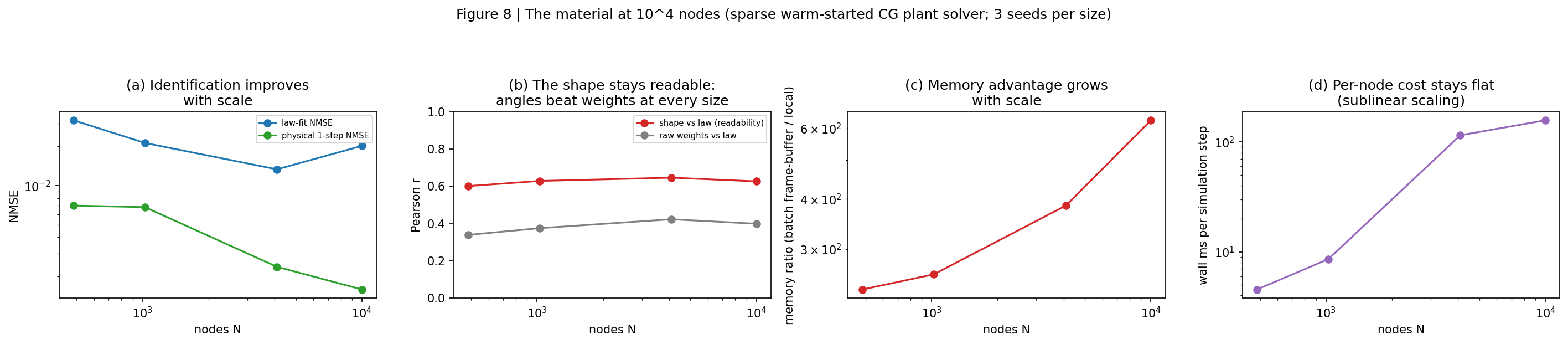
Scaling to 10,000 nodes: identification improves, memory advantage grows to 630x
10⁴ nodes · ~0.1 s/step

Compute you can hold

10,000 nodes learn at ~0.1 seconds per step on a laptop CPU, with ~630× less memory than a reservoir. Learning without a GPU — the compute that currently gates who gets to train AI.

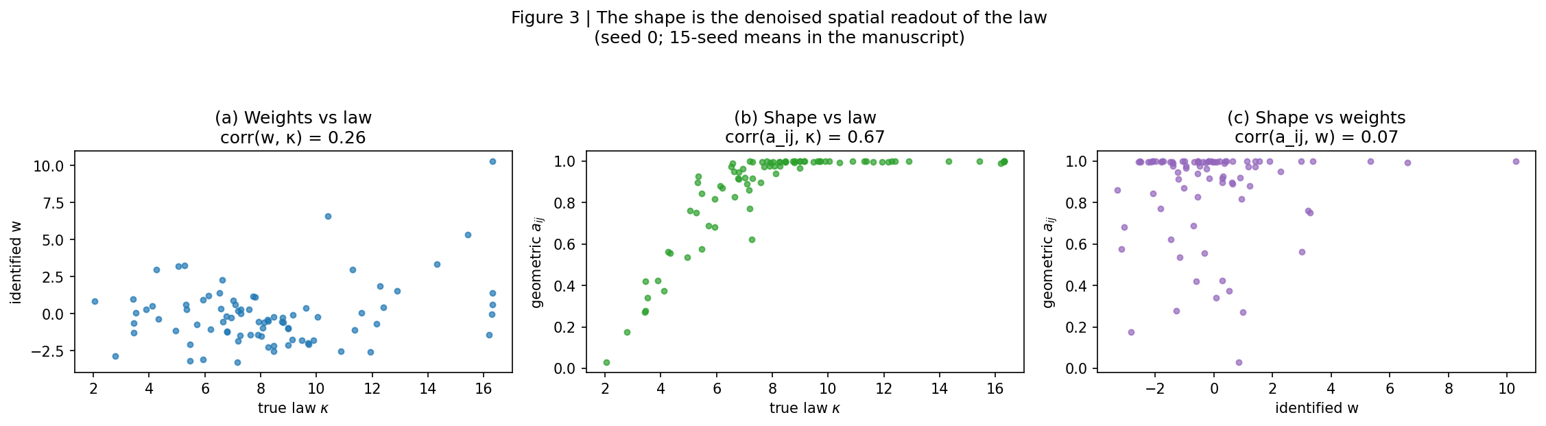
The shape reads back the law at r=0.64 vs r=0.35 for the raw weights
The shape is the readout

Mechanistic interpretability by construction

You watch what it learned — the geometry grows into the law (r = 0.64 vs 0.35 for raw weights). For safety-critical AI, inspectability is the architecture, not a post-hoc tool.

Real-data validation on the 277-year sunspot record: holdout law-fit, noise robustness, forecasts
481× & 22× below FD

Laws from noisy, sparse data

Two real physical records — solar activity and El Niño — identified at 481× and 22× lower holdout error than finite differences, flat under 50% added noise, and 5.3× better than a trained LSTM at 10% of the data. Climate, materials, biology: the law extraction regimes where data is scarce and dirty.

Steady-state routing: the learned shape redirects flux from source to sink
A substrate, not just software

Designed to be what a material does

Strictly local, O(E)-per-step updates are the update rule of physical hardware — analog circuits, neuromorphic chips. This is the paper's roadmap: the same weak form, running on real voltages.

Second real benchmark: NINO3.4 El Nino SST - at 10% of the data the law beats the trained LSTM 5.3x
One law, two worlds

Generalization as a property, not a hope

The identical identifier — unmodified — transfers across two independent physical systems and routes a maze it never saw at exactly oracle-level steps. Transfer measured, not assumed.

These are the directions the architecture opens — not claims it has met. Every number on this page is measured; every vision above it is a measured capability pointed at a problem. The honest boundary is stated in the papers: the same long-horizon forecast gap every derivative-law learner faces, and a hardware demo that remains the decisive next experiment.

Approach

Two channels of computation. Each neuron carries three state variables: an activation \(u_i\), a slow chemical state \(c_i\), and a 3D structural vector \(\hat{\mathbf v}_i\). The weight channel is identified locally and in-stream. Instead of finite-difference derivatives — which amplify noise by \(2\sigma^2/\Delta t^2\) — the network integrates against a localized exponential test function \(\psi(s)=\lambda e^{-\lambda s}\), throwing the derivative off the noisy data and onto the known, clean test function (an IIR spacetime weak form). A per-node recursive least-squares loop then contracts the local coupling law at the observation-noise floor:

\[ \widehat{\partial_t u} \;=\; \frac{\int (\partial_s\psi)\,u\,\mathrm ds}{\int \psi\,\mathrm ds}, \qquad\qquad w_{k+1} = w_k + \frac{P_k\,\phi_k}{1+\phi_k^{\!\top}P_k\phi_k}\,\big(y_k-\phi_k^{\!\top}w_k\big) \]

The angle channel is a deterministic nematic consensus: each structural vector rotates toward the coupling-weighted mean of its neighbors, gated by the chemical field so geometry grows only where the chemistry potentiates it:

\[ \hat{\mathbf v}_i \;\leftarrow\; \mathrm{norm}\!\Big(\hat{\mathbf v}_i \;+\; \eta_g\, c_i \sum_{j\in\mathcal N(i)} \kappa_{ij}\,\hat{\mathbf v}_j\Big) \]

The channels meet in the effective connection — weights say how strongly, angles say where:

\[ \kappa_{ij} \;=\; w_{ij}\;\cdot\; c_{ij}\;\cdot\; (\hat{\mathbf v}_i\!\cdot\!\hat{\mathbf v}_j) \]

The result is a material that learns its own physics and then grows into it — the emergent shape is a spatially coherent, denoised readout of the mechanism the weights encode edge-by-edge in multicollinear noise.
Architecture: fast electrical continuum, slow chemical continuum, IIR weak-form identifier, morphogenesis layer
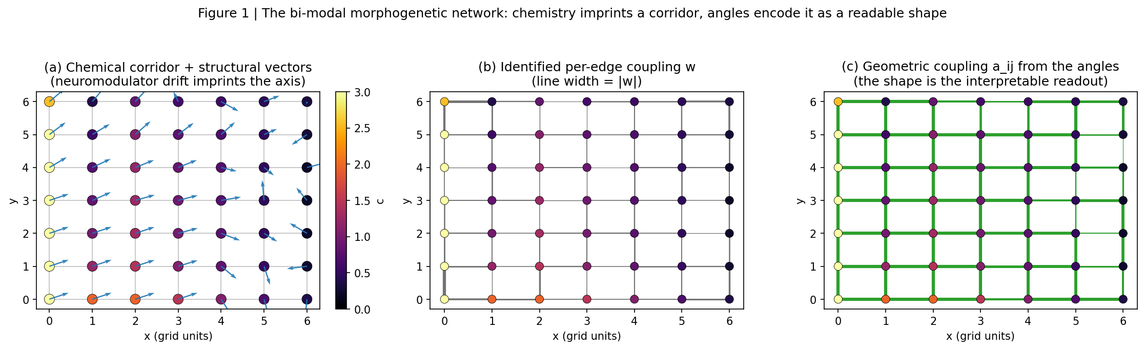
Figure 1. Architecture — fast electrical continuum (implicit graph diffusion), slow chemical continuum (reaction–diffusion–advection), IIR spacetime weak form, per-node streaming RLS, and nematic-consensus morphogenesis.
Learning curves: streaming weak form vs streaming-global RLS vs batch oracle vs finite-difference RLS
Figure 2. Law-fit NMSE vs time (15 seeds, 5% noise, regime-switching drift): per-node locality itself earns most of the advantage over the best streaming-global RLS (0.038 ± 0.009 vs 0.339).
The angle field reads back the true law better than the raw weights
Figure 3. The shape is the interpretable spectrum: the angle field reads back the true law at r = 0.64 vs r = 0.35 for the raw weights (better in 14/15 seeds) — the weights are multicollinear noise per edge, while the shape is their spatially coherent aggregate.

Results

Controlled baselines (streaming-global RLS, batch weak-form SINDy, finite-difference RLS), a full ablation, 15 seeds, and a playable maze: each mechanism earns its place, and the two channels are complementary — each alone is unreliable; the composed material is not.

8.9×

Locality, isolated

held-out NMSE 0.038 ± 0.009 vs 0.339 for the best streaming-global RLS (15 seeds)

6/8 → 0/8

Routing ablation

positive-transmission seeds with the learned geometric channel on → off

12/15

Corridor gain

seeds where learned geometry raises axial corridor transmission

r = 0.5–0.63

Shape encodes the law

corr(shape, discovered law) vs 0.08 for raw weights — geometry denoises the mechanism

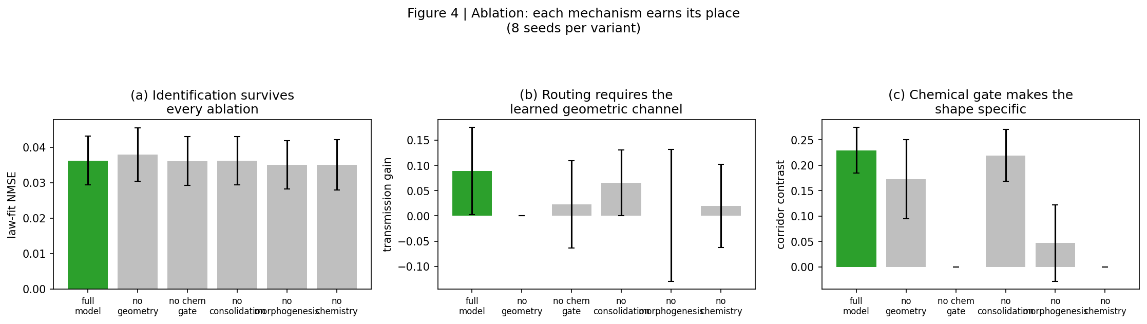
Ablation: identification survives every ablation; routing strictly requires the learned geometric channel
Figure 4. Ablation (8 seeds × 6 variants). Identification survives every ablation (NMSE flat at ~0.036); routing collapses without the learned geometric channel; the chemical gate is what makes the shape specific.
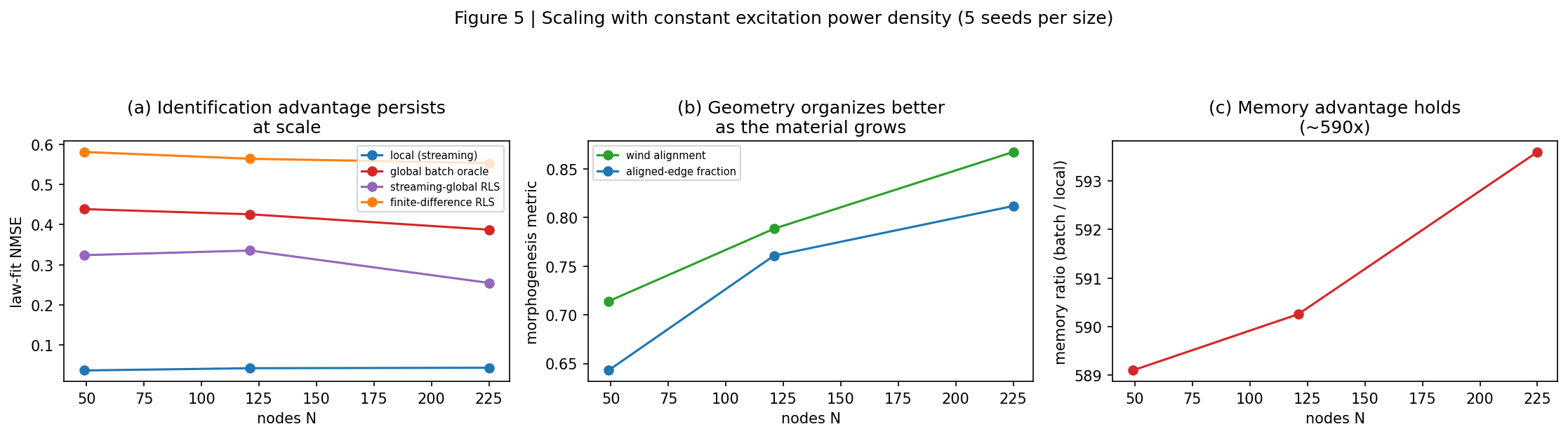
Scaling: identification advantage persists from 49 to 225 nodes; self-organization improves with scale
Figure 5. Scaling (5 seeds × 3 grid sizes, constant power density). The identification advantage persists from 49 → 225 nodes while self-organization coherence improves.
Learned geometry routes the flow along the corridor
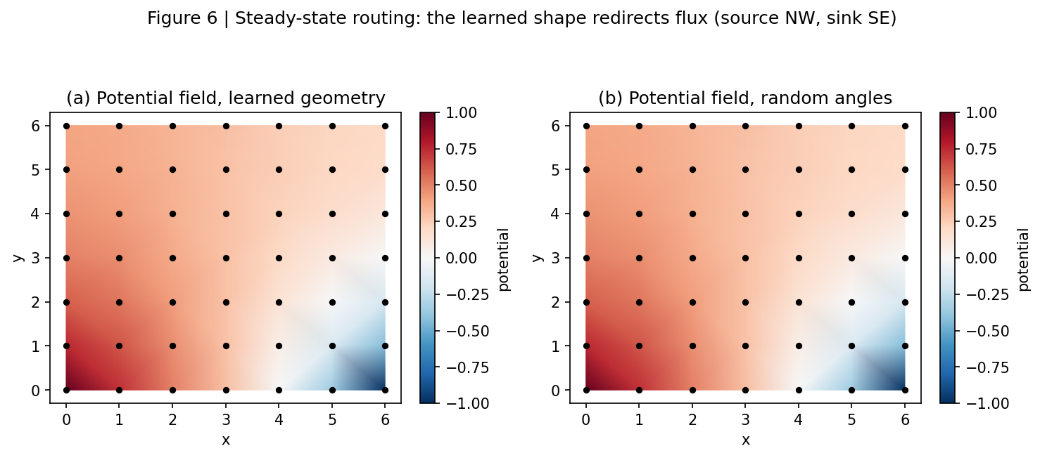
Figure 6. Geometry routes the physics: steady-state flux follows the learned geometry, and axial corridor transmission rises over the identical network with unlearned angles.

Real data — two physical systems, one unmodified identifier

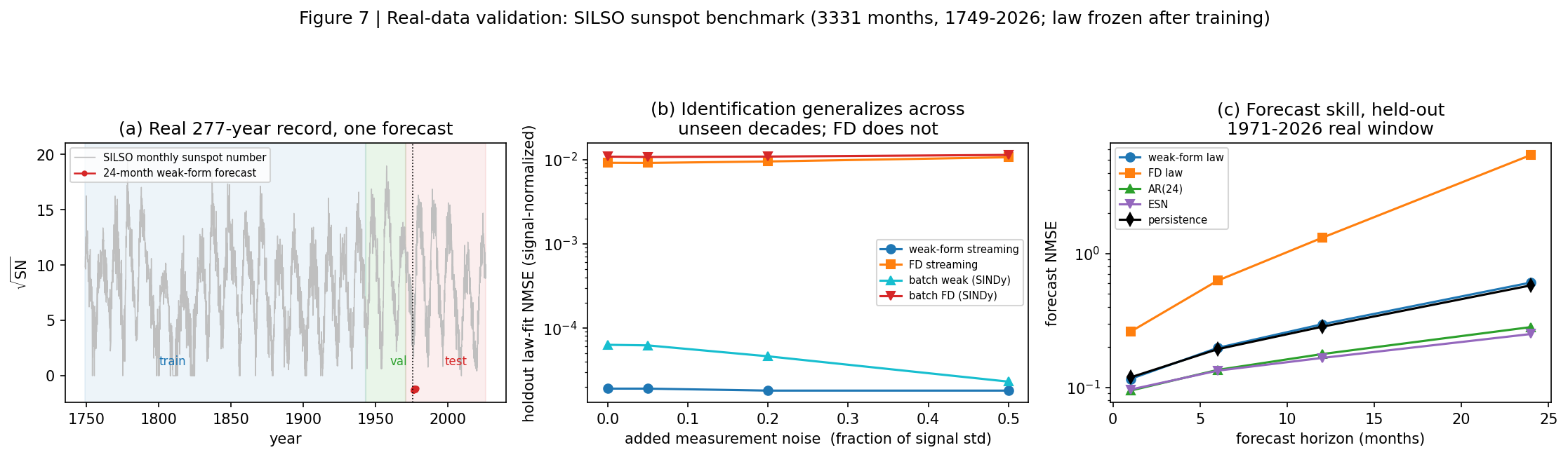
The 277-year sunspot record (SILSO). The identification layer, unmodified, runs on 3,331 real monthly observations (1749–2026), delay-embedded as a ring of 24 lag nodes. The law is frozen after training and evaluated on an unseen 27-year window (1991–2023); hyperparameters are tuned only on a validation window and nothing downstream is retrained. The weak form identifies the hidden law at 481× lower holdout error than finite-difference streaming, flat under 50% added measurement noise.

Real-data validation: holdout law-fit across unseen decades, noise robustness, forecasts vs horizon
Figure 7. (a) the record with train/val/test split; (b) holdout law-fit NMSE vs added measurement noise — the weak form stays flat at ~1.9e-5 from 0 → 50% noise while finite-difference degrades; (c) forecast NMSE vs horizon.

Forecast NMSE by horizon, held-out 1991–2023. The honest boundary, stated plainly: the weak form is a derivative law — it beats every finite-difference identification at every horizon and persistence at 1 month, while AR/ESN/LSTM, which fit the level directly, lead at long horizons. Numbers from real_benchmark.json.

horizonweak form (this work)FD streamingbatch weakbatch FDAR(24)ESNLSTMpersistence
1 mo0.1160.2600.1170.1870.0950.0960.0930.119
6 mo0.1970.6270.2040.3090.1350.1330.1300.193
12 mo0.2961.3100.3100.5270.1770.1660.1700.284
24 mo0.6075.4490.6281.5610.2820.2510.2890.578

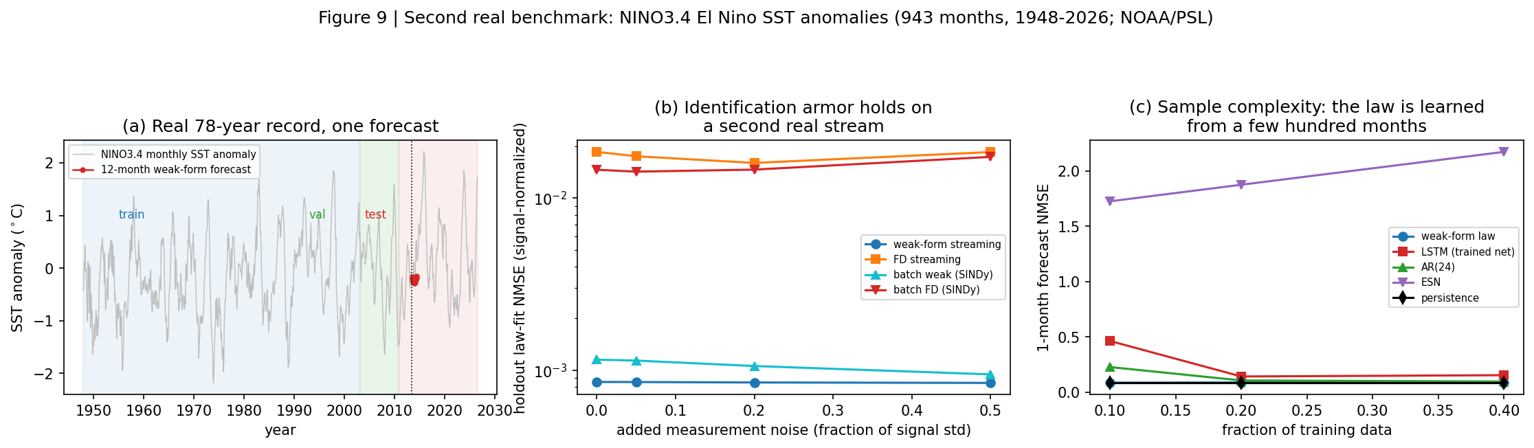
A second real stream — El Niño SST (ENSO). The protocol, unchanged, on the NINO3.4 monthly sea-surface temperature anomaly index (943 real observations, 1948–2026; NOAA/PSL) — a different physical system, no re-tuning. The armor transfers (22× below FD, flat under 50% noise), the deep-learning boundary flips (weak beats the trained LSTM at 6- and 12-month forecasts), and the sample-complexity gap is the headline: at 10% of the data the weak-form law is 5.3× better than the trained LSTM at one-month forecasts (0.087 vs 0.464) while the reservoir collapses (1.73).

Second real benchmark: NINO3.4 El Nino SST — identification armor, forecast skill, low-data sample complexity
Figure 8. (a) record with split; (b) holdout law-fit vs added noise — flat under 50% noise, ~22× below FD; (c) one-month NMSE as training data shrinks — at 10% of the record the weak-form law is 5.3× better than the trained LSTM while the reservoir collapses.
481× / 22×

Identification armor

vs finite-difference streaming on sunspots and ENSO; flat under 50% added noise on both

5.3×

Better than the LSTM

one-month NMSE at 10% of the data (0.087 vs 0.464); wins 6- and 12-month forecasts at full data

126 KB

Law state

vs 1.25 MB reservoir at comparable or better long-horizon behavior

3.3× / 1.35×

Streaming vs batch

exponential forgetting adapts to the recent regime on both real records

The material at 10,000 nodes

The dense plant solver is O(N3) per step; a sparse warm-started conjugate-gradient solve (the relaxation a physical network performs, exact to 1e-9 and verified identical to the dense solve) makes the step O(E). From 484 to 10,000 nodes: identification improves with scale (law-fit 0.032 → 0.020), the shape stays readable at every size (r = 0.60–0.65 vs 0.34–0.42 for the raw weights), the memory advantage grows (~240× → ~630×), and per-node cost is sublinear. The honest limitation: the corridor-routing contrast saturates at 103–104 nodes.

Scaling to 10,000 nodes: identification improves, shape readability persists, memory advantage grows, per-node cost sublinear
Figure 9. (a) identification improves with scale; (b) the angle field beats the raw weights at every size; (c) memory advantage grows; (d) per-node cost sublinear.

Theory — what the loop guarantees

Four theorems with proofs in the paper and numerical verification in theory.json:

(T1) Noise floor. The weak-form derivative estimate has variance converging to \(\lambda^2\sigma^2\), independent of the sampling interval — while finite differences amplify as \(2\sigma^2/\Delta t^2\). Measured: a 2.2×10⁵× gap at dt = 10−3, ratios 0.998–1.000 against theory.

(T2) Contraction. Streaming RLS contracts under persistence of excitation, with tracking error linear in the law-drift rate — a 238× reduction, halved in 5 samples.

(T3) Monotone self-organization. Angulation is monotone ascent on the alignment functional: alignment rises 0.511 → 0.878, never decreasing.

(T4) The closed loop. Morphogenesis is the contraction plus an O(ηe) perturbation — the shape grows while identification is perturbed by only ~7%.

Run it yourself

Python 3.9+; only numpy, matplotlib, and (for the game clip) Pillow are required. Every paper number is produced by these scripts from the committed result files.

pip install -r requirements.txt
python run_experiments.py --task sweep     --seeds 15 --T 4000 --out results.json
python run_experiments.py --task ablation --seeds 8  --T 4000 --out ablation.json
python run_experiments.py --task scale    --seeds 5  --T 4000 --sizes 7x7,11x11,15x15 --out scaling.json
python scale_large.py --sizes 22x22,32x32,64x64,100x100 --seeds 3 --T 1500 --out scaling_large.json
python real_benchmark.py --dataset sunspot --out real_benchmark.json
python real_benchmark.py --dataset enso    --out real_benchmark_enso.json
python theory.py
python flowgame.py --episodes 4 --out game           # the maze game + animated clip
python make_figures.py                               # paper figures 1-9
python make_paradigm_fig.py                          # the angle-paradigm hero figure
python test_biomaterial_net.py                       # 12 sanity tests

See the repository for the full README, methods, baselines, and eight documented failure modes. LaTeX sources for both papers (nmi_paper.tex, ieee_paper.tex) are included and regenerate with pdflatex.

Citation (BibTeX)

@article{singh2026morphogenetic,
  title   = {Morphogenetic Bi-Modal Networks: Two Channels of Computation -- Weights and Angles},
  author  = {Singh, Sehaj},
  year    = {2026},
  note    = {Gradient-free local learning; IIR spacetime weak form; angle-channel morphogenesis},
  url     = {https://github.com/sehajr-singhs/morphogenetic-bimodal-networks}
}