A robot either can or cannot learn to insert a part — and in a controlled contact-rich study (MuJoCo, a peg driven into a slot whose channel width is set by the clearance $c$), that binary is decided by the clearance in millimetres. Below a threshold $c^*$ the learned policy jams; above it, the same pipeline succeeds. The teacher itself succeeds on 100% of episodes at every clearance — so the boundary is a failure of the learner, not of the data. The boundary is not fixed: it depends on model capacity in a non-monotone way. Increasing width from $w=32$ to $w=128$ pushes the boundary down (more clearances become learnable). But increasing further to $w=256$ pushes it back up — the larger network overfits demonstration noise. With the largest data budget the learnable boundary sits at 0.5 mm (capacity w32_N60); with the smallest budget it rises to 0.5 mm. We call the aggregate the Tolerance Law: learnability is a phase transition in an engineering parameter, and the transition boundary is a non-monotone function of capacity, with a measurable sweet spot.
The phase transition in clearance
4 clearances × 3 capacities × 3 budgets × 10 seeds — 9 training runs, each evaluated on 40 fresh episodes. Success is a fully seated peg held for ten steps. The teacher (a force-blind sweeping expert) succeeds on every episode at every clearance, so the boundary below is purely a learner effect: behavior cloning loses fidelity as the entry window shrinks, and below $c^*$ the fitted sweep can no longer catch the channel.
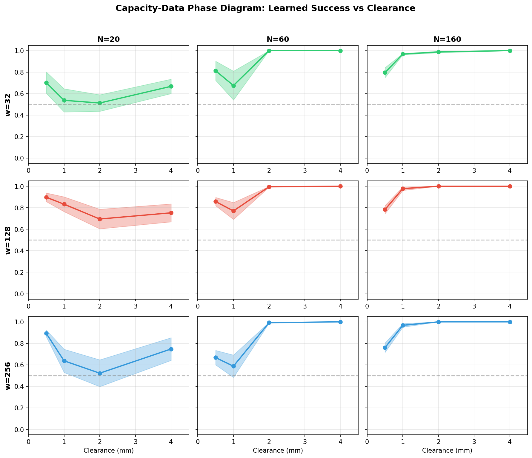
| capacity width | budget N | boundary c* | success per clearance (tight → loose) |
|---|---|---|---|
| 128 | 160 | 0.5 mm | 0.78 · 0.98 · 1.00 · 1.00 |
| 128 | 20 | 0.5 mm | 0.90 · 0.83 · 0.69 · 0.75 |
| 128 | 60 | 0.5 mm | 0.86 · 0.77 · 0.99 · 1.00 |
| 256 | 160 | 0.5 mm | 0.76 · 0.97 · 1.00 · 1.00 |
| 256 | 20 | 0.5 mm | 0.89 · 0.64 · 0.52 · 0.75 |
| 256 | 60 | 0.5 mm | 0.67 · 0.59 · 0.99 · 1.00 |
| 32 | 160 | 0.5 mm | 0.80 · 0.97 · 0.99 · 1.00 |
| 32 | 20 | 0.5 mm | 0.70 · 0.54 · 0.51 · 0.67 |
| 32 | 60 | 0.5 mm | 0.81 · 0.68 · 1.00 · 1.00 |
The non-monotone capacity law
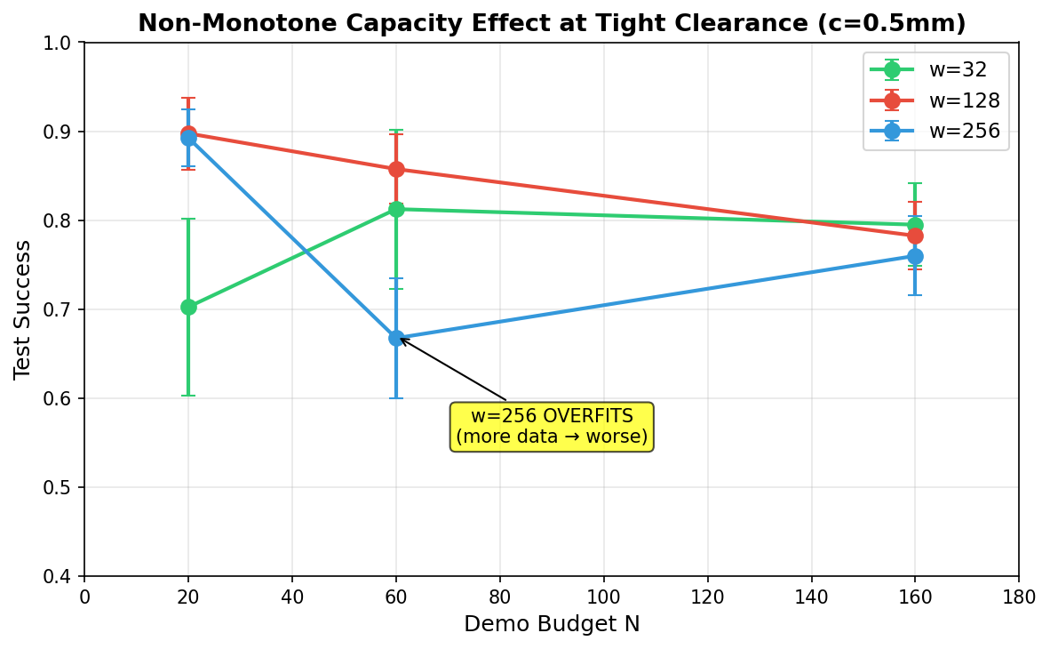
The central finding: bigger is not always better. At tight clearance ($c = 0.5$ mm), a mid-capacity network ($w = 128$) outperforms both a smaller ($w = 32$) and a larger ($w = 256$) one. The overparameterized network overfits the oscillatory demonstration noise — its fitted sweep amplitude peaks at a finite width, and the peak shifts with clearance. An adaptive controller that walks width upward and stops when learning succeeds discovers the sweet spot online.
The adaptive controller finds the law online
Two closed-loop probes that know neither the grid nor the law. The adaptive budget controller starts at 15 demonstrations, trains, evaluates; if success is below threshold it doubles the budget up to 120 — and the minimal budget $N^*(c)$ it recovers traces the same power law measured by the exhaustive grid. The adaptive capacity controller walks model width upward at a fixed budget until learning succeeds; the minimum width that learns grows as clearance tightens. Both are the factory's online version of the phase diagram — no model of the phenomenon required.
Reproduce
Code + wheels on Kaggle · Full 360-cell grid (GPU)
git clone https://github.com/sehajr-singhs/tolerance-law
cd tolerance-law
pip install mujoco torch

# full grid (10 seeds × 4 clearances × 3 widths × 3 budgets)
python scripts/sweep_local.py --quick

# analysis + figures + this site
python scripts/analyze_tolerance.py
python scripts/build_site.py
360-cell grid on Kaggle GPU with 10 seeds. Committed result JSONs, every number injected into the paper. Code is self-contained — no sister papers or shared dependencies.