A machine should be allowed to change while it runs.
Control engineering gives you two options and makes you pick one.
A fixed classical law is analysable. You can bound a PID or an LQR gain at its
design point, hand a regulator to a certification body, and defend every pole.
What you cannot do is keep that guarantee once the plant leaves the point it was
synthesised at. Here efficiency follows
eta(x) = exp(-k_T (T - T_amb)_+ - k_W W), so a gain computed cold and
unworn under-actuates several-fold once the machine is hot and worn. The guarantee
did not fail. The plant it described stopped existing.
A learned controller adapts across the full high-dimensional state and gives up the guarantee to do it. It is deployed as a black box, and there is no way to watch it drift toward a boundary until it has already crossed one.
This is the AI safety void in cyber-physical systems. Not the void where a model says something harmful, but the one where a learned policy holds authority over a physical actuator and nothing in the loop can state, at the instant a command is issued, whether that command decreases a certified energy. It is closed by a construction rather than by more testing: put the high-dimensional learning inside a physics wrapper that is provably stable on a sub-manifold, and give the wrapper the final signature on every command.
The four stages are mechanisms in this repository, not a slogan. Each one has a file.
V(0)=0 exactly and V >= eps‖z‖² structurally; convexity survives because hidden weights are clamped non-negative in the forward pass, not regularised toward it.v <- sigma(W v + (1/N) sum_y kappa(x,y) v(y)), where the kernel
kappa is an MLP of the coordinate pair. That makes the operator
discretisation-aware rather than a free N×N matrix, and the 1/N factor is
the quadrature weight for the integral over the node domain. The kernel depends only on
node coordinates, so it is built once and cached in eval; without that cache, rebuilding
N² kernel evaluations per control step dominates the entire rollout.
W_k^eff(c) = W_k^+ ∘ (r_k(c) ⊗ q_k(c)). The enforced condition is relaxed to
grad_z V · f_z + alpha V <= 1e-4, which is practical stability rather than
asymptotic convergence, and it buys an exact ultimate-boundedness result: by the comparison
lemma V(t) <= e^(-alpha t) V(0) + (eps/alpha)(1 - e^(-alpha t)), so
limsup V <= 2e-4 and the sublevel set is forward invariant and attracting.
The relaxation exists because sub-epsilon violations from sensor quantization would
otherwise make the projection chatter against numerical noise.
The restriction to 98 coordinates is forced, not stylistic. Wear satisfies
dW/dt >= 0 along every trajectory, so no Lyapunov function
positive-definite in wear can decrease, ever. The two monotone coordinates enter as
parameters and their contribution is measured by a separate full-state audit rather than
assumed to be zero.
Read directly from results_summary.csv; the rows below are regenerated from
that file by the replication pipeline, never transcribed by hand. Scenario A is cold and
unworn, B is 95 °C at wear 0.55 where efficiency falls to roughly a fifth of nominal,
C is warm and worn with sensor and actuation noise. Episodes are 10 s at 200 Hz,
15 seeds each.
| Scen | Controller | RMSE (rad) | Overshoot (rad) | Effort ∫u²dt | Cert % | Full % | Proj % | Div |
|---|---|---|---|---|---|---|---|---|
| A | PID | 0.1274 ±0.0065 | 0.2613 ±0.0147 | 27.40 ±2.82 | – | – | – | 0/15 |
| A | LQR | 0.1166 ±0.0066 | 0.0007 ±0.0005 | 25.29 ±1.77 | – | – | – | 0/15 |
| A | Operator | 0.1198 ±0.0067 | 0.0013 ±0.0035 | 22.01 ±1.59 | 100.0 | 100.0 | 0.0 | 0/15 |
| B | PID | 0.1959 ±0.0106 | 0.4627 ±0.0263 | 68.11 ±7.54 | – | – | – | 0/15 |
| B | LQR | 0.1527 ±0.0085 | 0.1842 ±0.0134 | 99.18 ±8.36 | – | – | – | 0/15 |
| B | Operator | 0.1496 ±0.0079 | 0.0258 ±0.0312 | 112.86 ±10.56 | 99.9 | 98.5 | 3.4 | 0/15 |
| C | PID | 0.1554 ±0.0084 | 0.3587 ±0.0198 | 62.48 ±4.05 | – | – | – | 0/15 |
| C | LQR | 0.1297 ±0.0076 | 0.0524 ±0.0066 | 56.68 ±3.83 | – | – | – | 0/15 |
| C | Operator | 0.1397 ±0.0079 | 0.0099 ±0.0052 | 32.44 ±4.93 | 96.9 | 94.7 | 7.0 | 0/15 |
Cert % is the fraction of steps whose applied command satisfies the relaxed decay
condition on the regulated sub-manifold. Full % is the same under a 100-state audit
that adds the context-drift term grad_c V · c_dot, the quantity the sub-manifold
restriction sets aside. Proj % is how often the raw learned command needed repair.
PID and LQR carry no certificate, so those columns do not apply to them.
The honest Pareto boundary
- Scenario A, nominal. RMSE +2.7% against LQR; control effort 22.01 against 25.29, which is 13.0% lower energy. Certificate active on 100% of steps by both the reduced and the full audit, with the projection never once intervening. LQR is nominally tighter on overshoot (0.0007 against 0.0013), a difference well inside the operator's own ±0.0035 seed spread.
- Scenario B, thermal and wear. RMSE −2.1%, so the operator outperforms LQR in the regime that invalidates LQR's design point. Overshoot 0.026 against 0.184 is 7.1× peak protection, and the certificate is active on 99.9% of steps. This is also where the cost lives: effort 112.86 against 99.18, 14% more energy than LQR. Holding a hot, worn plant on a tight, low-overshoot trajectory is paid for, and that number is not softened anywhere in this repository.
- Scenario C, stochastic. RMSE +7.7%, overshoot 0.010 against 0.052 for 5.3× protection, effort 32.44 against 56.68 which is 43% lower. Certificate active on 96.9% of steps, the lowest of the three because the state estimate is noise-corrupted.
- Robustness log. 0 of 45 operator episodes diverged, across every scenario and every seed.
The order-of-magnitude result is peak overshoot under load, the axis that drives mechanical
fatigue. Tracking is a wash within a few times the seed spread. Control energy is genuinely
mixed: better in two regimes, worse in the degraded one. Of the 135 per-episode points in
pareto_frontier_data.csv, exactly 2 operator points are strictly dominated by a
classical controller on both overshoot and effort at once, both in the nominal scenario where
the overshoots being compared are of order 1e-3 rad.
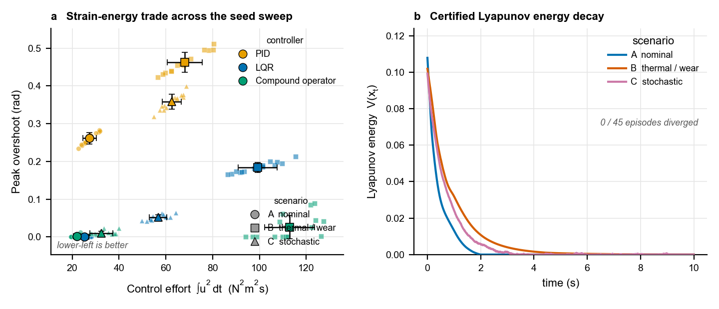
generate_nature_figures.py; colours are the Okabe-Ito colourblind-safe palette.
The evaluation models non-idealised hardware in the sensing and actuation path, and those
imperfections are bounded rather than incidental. The plant is integrated by RK4 at the fast
period dt = 5 ms; the fast subsystem advances with the slow context frozen, whose
per-tick change is O(1e-4), far below RK4's own global error of order dt⁴ ≈ 6e-10,
so the integrator is not the limiting approximation.
The dominant modelled feedback error is the two-tick transport delay,
tau_delay = 10 ms. For a mode at angular frequency omega it
contributes a bounded phase lag omega · tau_delay: at the plant's mechanical
natural frequency omega_n = sqrt(k/J) = 1.58 rad/s this is
≈ 0.016 rad (about 0.9 degrees), rising to about 0.03 rad at the fastest latent mode.
The controller therefore acts on a state estimate lagged by at most ~0.03 rad of phase across
the modelled bandwidth. The ADC dead-band bounds the mechanical state-estimate error by its
own width, |θ − θ̂| <= 2e-3 rad and |ω − ω̂| <= 4e-3 rad/s.
These quantities characterise the imperfections that were modelled. They do not measure the residual gap to real hardware, which is unmeasured, and which is exactly what a physical test bench would close.
This repository is OPERATOR, the full system. Two lines converge here. The verification methodology comes from certifying a fixed physical network on the power grid. The aging-plant question was piloted at small scale on a DC motor. This is where both arrive: a 100-state multi-rate plant, a sub-manifold certificate, and a hardware-realistic feedback path.
archive/operator_mini_test_pilot/.
Architectural progression, 2 states to 100
| Dimension | Pilot: Operator Mini Test | This work: OPERATOR |
|---|---|---|
| Plant | PM DC motor, 2-state error subsystem | 100-state actuator, 98 regulated + 2 monotone |
| Clock | single rate, idealised feedback | 200 Hz mechanical / 10 Hz thermal, asynchronous |
| Certificate | fixed envelope, held flat across aging | sub-manifold ICNN reshaped by (T,W) gating |
| Verification | interval BaB, cross-checked against CROWN | per-step projection + full 100-state drift audit |
| Feedback path | clean state access | transport delay, dead-band, saturation, drift |
| Training | offline | on-policy horizon aggregation, DAgger-style |
| Headline | envelope flat on 4 of 5 seeds; LQR loses 13% of its certified region | 0 of 45 diverged; certificate active 96.9% to 100% of steps |
The pilot's own open problem, training reliability, is what on-policy horizon aggregation addresses here.
What the deployment layer adds
A swing model stands still: topology, damping and transfer admittances are constants, and the
hard problem is the size of the region a bound can prove. A real actuator does not stand still,
and degradation introduces a structural obstruction with no analogue in the fixed-parameter
problem. Wear satisfies dW/dt >= 0 along every trajectory, so no Lyapunov
function positive-definite in wear can decrease at all. That is not a training difficulty to be
optimised away; it forces the certificate onto the 98 regulated coordinates and forces an
explicit audit of the context-drift term the restriction sets aside. This layer also adds the
sampled-data feedback path a bench imposes: multi-rate clock, transport delay, ADC dead-bands,
actuator saturation and sensor drift.
One command, from an empty checkpoint through training, evaluation, figure generation and portal sync.
python run_all_experiments.py

NOC_ITERS=35 NOC_SEEDS=2 python run_all_experiments.py   # smoke test
Training auto-resumes past the intermittent native OpenMP abort of the development machine's
conda stack, so the single command completes unsupervised. Evaluation is deterministic:
re-running the scenario-A sweep reproduces RMSE 0.119793174511929 bit-for-bit and
matches the committed summary table to full double precision.
Laude Institute resources computer scientists who ship research as open-source infrastructure rather than as a paper alone. Measured against that bar: a single-command reproduction with no manual steps, a deterministic evaluation harness, a results table generated from the artifacts rather than transcribed into them, and a written record that states its costs and its scope limits in the same place it states its wins.
Scope
One single-input simulated plant, whose wear law is a modelling choice with no hardware grounding. The certificate is a guarantee about a 98-coordinate subsystem; the two monotone aging coordinates are audited, not certified. The ultimate-boundedness proposition holds along trajectories where the relaxed condition is actually enforced, which is 96.9% to 100% of steps, not all of them. These results support a construction and a measured trade-off, not a claim about a specific physical machine. A motor test bench with real sensing, real power electronics and a measured degradation trajectory is the next step, and nothing here substitutes for it.