stochastic-latent-bounds

Welcome!

Trajectories and the certified latent region — Latent-space view of the certified system: trajectories of the physical SDE pushed through the learned invertible transport `T`, the certified η-region (green) and the noise ball promised by the certificate. Generated by `tools/gifgen.py` from the committed arm4 checkpoint.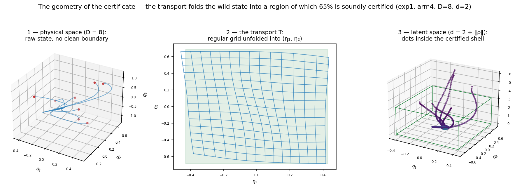

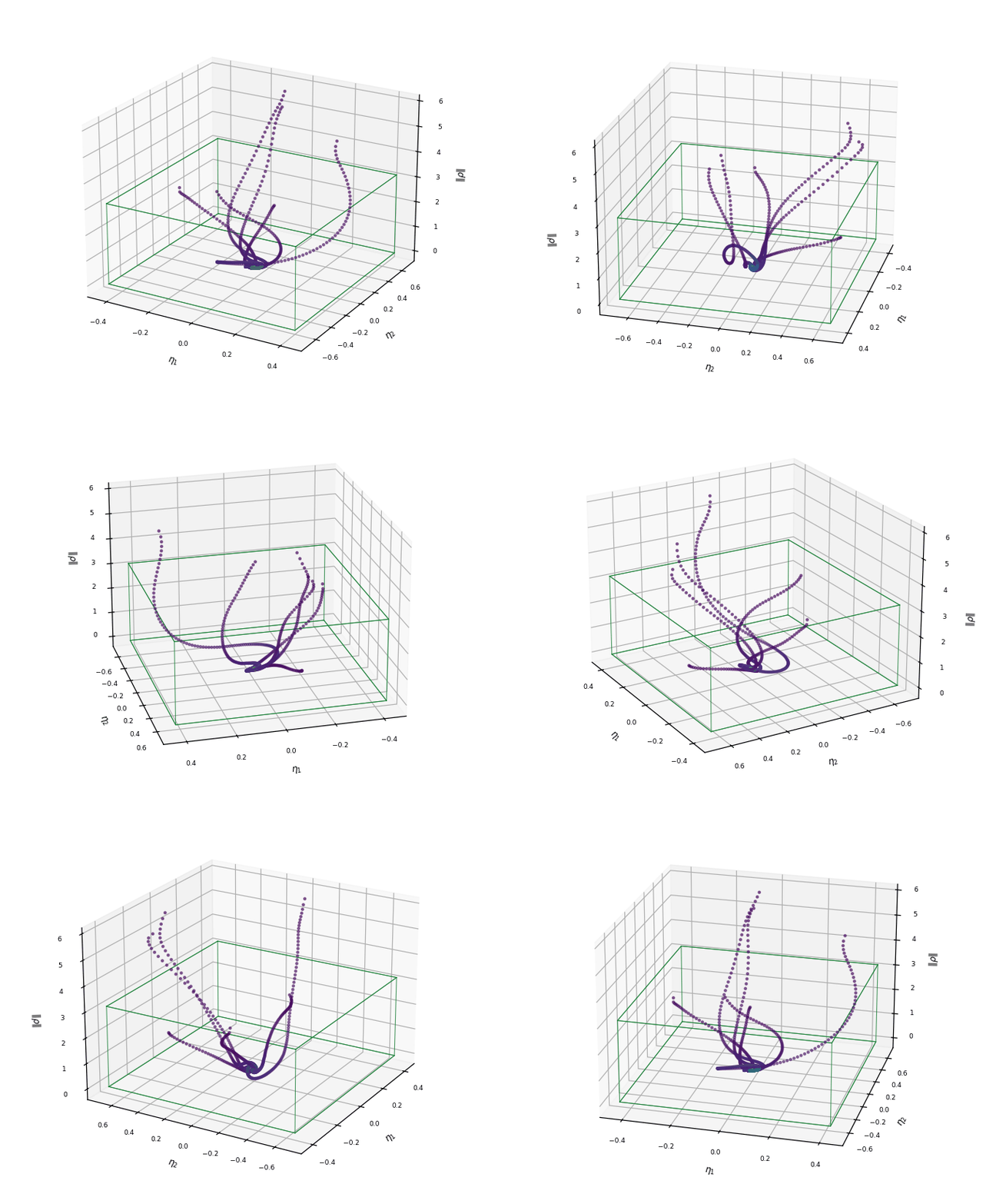The three-frame geometry: physical spaghetti, the transport unfolding, dotted trajectories inside the certified shell — The geometry of the certificate in three frames. Left: the raw physical state of the 4‑link arm (first three joint angles) — wild, noisy, no clean boundary. Middle: the learned invertible transport unfolding a regular physical grid into latent coordinates — the “hands” that straighten the dynamics; the green box is the certified η‑region. Right: the same trajectories as moving dots in latent space (η₁, η₂, ‖ρ‖) — they bounce around inside the certified shell but never puncture it. The orbiting view: Generated by `tools/viz3d.py`.

Orbiting view of the certified shell — The geometry of the certificate in three frames. Left: the raw physical state of the 4‑link arm (first three joint angles) — wild, noisy, no clean boundary. Middle: the learned invertible transport unfolding a regular physical grid into latent coordinates — the “hands” that straighten the dynamics; the green box is the certified η‑region. Right: the same trajectories as moving dots in latent space (η₁, η₂, ‖ρ‖) — they bounce around inside the certified shell but never puncture it. The orbiting view: Generated by `tools/viz3d.py`.

stochastic-latent-bounds turns a stochastic physical system into coordinates where a Lyapunov certificate is searchable: a learned, exactly invertible transport factors the state into a low‑dimensional certified factor and a transversal residual, and the certificate is verified by interval branch‑and‑bound — never assumed from samples.

64.9% vs 2%

learned transport vs PCA on the nonlinear plant (exp9) — random: 0%

59.1%

arm6 (d=3) certified — with 8× budget; effort tracks d, not D

8 / 0

unsafe swaps, naive vs gated, under real fleet aging

real domains: turbofan fleet, Beijing air, ETTm2 grid

tests: soundness, loaders, baselines, bootstrap statistics

±0.02

bootstrap CI half‑width on violation fractions (2048 probes)

stochastic Lyapunovinterval arithmeticinvertible transportsbranch & boundworld models

Classical certification does not scale: sum‑of‑squares and SMT methods collapse under the curse of dimensionality, while neural Lyapunov functions are usually validated only at sampled points. Every number published on this site is rendered from committed results/*.json produced by the committed code — the site cannot drift from what the experiments actually did.

Getting Started

Installation

git clone https://github.com/sehajr-singhs/stochastic-latent-bounds
cd stochastic-latent-bounds
pip install torch pytest

# soundness + tightness test suite (CPU, float64)
python -m pytest tests/ -q

Reproduce the results

python experiments/exp1_main.py          # factor vs full scaling (N-link arms)
python experiments/exp2_shadow.py        # gated hot-swap under plant drift
python experiments/exp3_tightness.py     # tight trace vs Cauchy-Schwarz
python experiments/exp4_realtrend.py     # NASA C-MAPSS fleet (Kaggle)
python experiments/exp5_airquality.py    # Beijing air quality (Kaggle)
python experiments/exp6_grid.py          # ETTm2 electricity transformer (Kaggle)
python experiments/exp7_baselines.py     # PCA / random-projection baselines, real data
python experiments/exp8_validation.py    # identification floors, CIs, ablations, seeds
python experiments/exp9_nonlinear.py     # learned vs fixed maps on the nonlinear plant
python tools/figures.py                  # regenerate figures from results/

How it works

The factorised certificate

An exactly invertible transport T (affine coupling layers, T(x*)=0 at the equilibrium) maps the physical state x to latent coordinates y=(eta, rho) — nothing is discarded, the map is a diffeomorphism. A certificate

W(y) = V(η) + κ ρᴹ Q ρ, L W + α W ≤ β + tol

is then verified over a region by worst‑first branch‑and‑bound. Factor mode searches only the d‑dimensional η‑box (the ρ‑side is handled by the Lyapunov metric in closed form); full mode searches all D coordinates. The soundness of the bound is what makes the difference a theorem, not a tune:

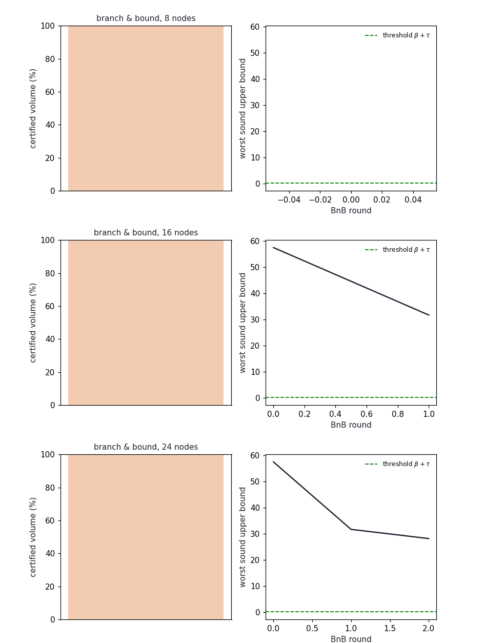
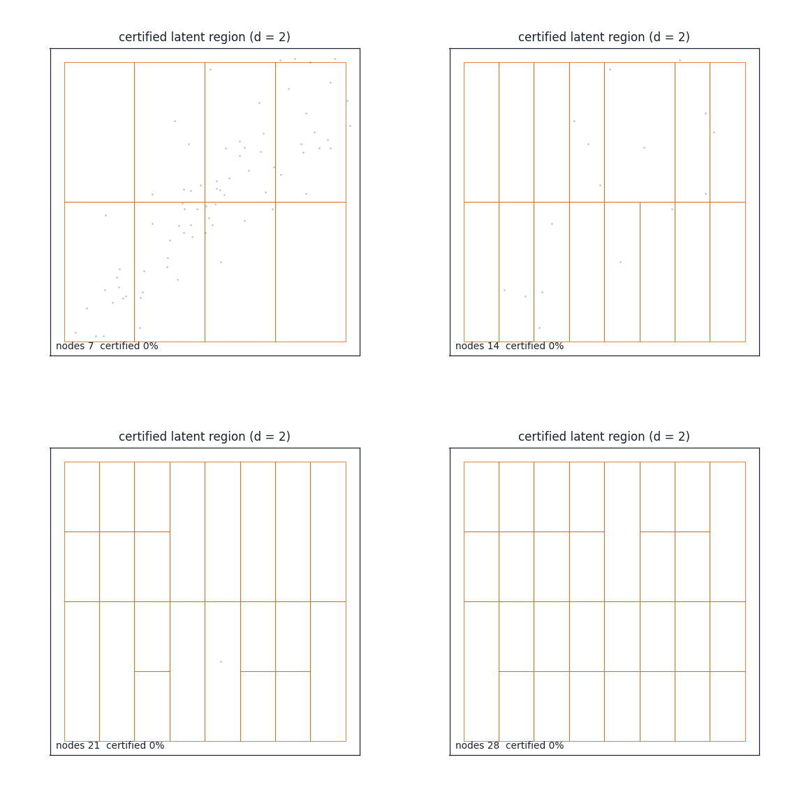
Branch-and-bound subdivision of the latent box — Worst‑first interval branch‑and‑bound subdividing the latent η‑box: red boxes still violate the sound upper bound on `L W + α W`, green boxes are certified against `β+tol`, grey boxes are resolved. Generated by `tools/gifgen.py` from the same committed checkpoint.

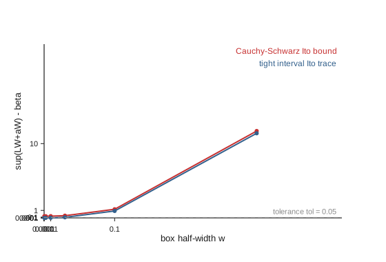
The bound on L W + α W is computed with sound enclosures: an exact interval Ito trace ½ tr(BBᴹ Hess W), centered (mean‑value) drift forms whose residual enclosure is a cascade (exact zeros on transversal columns, remainder quadratic in box radius), and outward rounding everywhere. Both choices make the bound converge under subdivision; the interval trace even converges to the exact generator on degenerate boxes, which is what makes certification near the origin possible at all.

The noise floor, honestly

With additive process noise the origin is not an equilibrium of the SDE: paths leave it immediately, so L W(0) = β > 0 and the classical condition certifies the empty set, always. The attainable statement is the thresholded certificate

L W + α W ≤ β + tol ⟹ E[W(t)] ≤ e⁻⁷t W₀ + ((β+tol)/α)(1 − e⁻⁷t)

i.e. exponential practical stability to an explicit noise ball of stationary radius (β+tol)/α. β is evaluated exactly at the origin; tol is explicit slack, reported rather than hidden.

What is verified, what is measured

Soundness is tested directly: across random boxes the sound bound must dominate the exact generator at every sampled interior point (tests/test_soundness.py).
Tightness is tested directly: a point box at the origin must reproduce β to 1e-6 — an assertion the Cauchy‑Schwarz bound structurally cannot pass.
The world model is scored against the analytic Ito push‑forward of the identified plant, so the learned‑vs‑exact gap is measured, including the Ito correction term most latent models silently absorb.
Online adaptation runs a shadow network behind a certified acceptance gate; unsafe swaps after a drift change are counted against the exact plant generator, so the gate's value is falsifiable.

Real physical data

Two real datasets, one pipeline, zero domain‑specific code:

NASA C‑MAPSS FD001 (turbofan fleet, 100 engines run to failure): per‑era Ornstein‑Uhlenbeck plants identified from real sensor trajectories; the aging drift moves the attractor 2.82 sd. Under that real drift the sound gate made 0 unsafe swaps while the naive gate accepted all 8 candidates — every one unsafe.
Beijing PRSA (multi‑site air quality, hourly 2013–2017): the drift event is the real seasonal regime shift (municipal heating season); the identified attractor moves 3.85 sd between regimes.

Results

Tightness sweep: bound excess versus box width — Excess of the sound bound over the noise floor β on shrinking boxes around the origin (log‑log). The Cauchy‑Schwarz Ito bound has irreducible slack and certifies nothing at any radius; the tight interval trace converges to the exact generator and certifies up to the tolerance line.

Full tables — scaling, hot‑swap traces, the effort ladder, the reactor and D=200 experiments — are on the results page. The full manuscript narrative is on the paper page. The mathematics (including the d‑vs‑D effort proposition) is in mathematics — now with the formal supplement: soundness of the certificate (Theorem 1), the noise‑floor lemma, convergence of the search (Theorem 2), robustness to plant mismatch (Theorem 3), and the d‑not‑D scaling law (Theorem 4), each with proof. The module map is in the API page.

Help

The certificate, the sound‑bound constructions and the counterexample‑guided retraining loop are documented in mathematics; module‑by‑module roles in the API map. Source: github.com/sehajr-singhs/stochastic-latent-bounds.