The thesis
Every engineered system is a graph. A truss is joints connected by members. A power grid is buses connected by lines. A molecule is atoms connected by bonds. A pipe network is junctions connected by segments. A heat exchanger is nodes connected by thermal paths. A vibrating structure is masses connected by springs.
GNoME-Mfg collapses all of these into one message-passing backbone and attaches a domain readout per physical quantity. The result is a single codebase that predicts seven different physics regimes instead of seven bespoke solvers.
The engineering effort was not the architecture. It was debugging the real failure modes that make models silently worse than predicting the average. Five bugs, five fixes, five honest numbers — documented because the failures are the roadmap.
Architecture
Two message-passing families handle the two geometric regimes. A shared backbone processes any graph. A domain-specific readout predicts the physical quantity.
nodes + edges + physics
truss, molecule
circuit, pipe, heat
per-quantity head
| Layer family | Geometric regime | Used for |
|---|---|---|
EquivariantMPLayer | Scalar + vector channels | Truss displacement, molecular energy |
MessagePassingLayer | Generic node features | Circuit angles, pipe pressure, heat temperature, vibration, acoustic |
Each domain model is a three-layer stack plus a small readout head. Targets are z-scored to unit variance before training — not cosmetic, but structural: the physical scales differ by ten orders of magnitude (metres vs pascals vs kelvin). Without standardization, the unscaled loss is dominated by whichever quantity has the largest variance.
Results
R² = 1 − NRMSE² on held-out graphs. R² = 1 is perfect, R² = 0 is the trivial mean predictor, and negative R² means the model is worse than predicting the average.
| Domain | Predicted quantity | R² | Status |
|---|---|---|---|
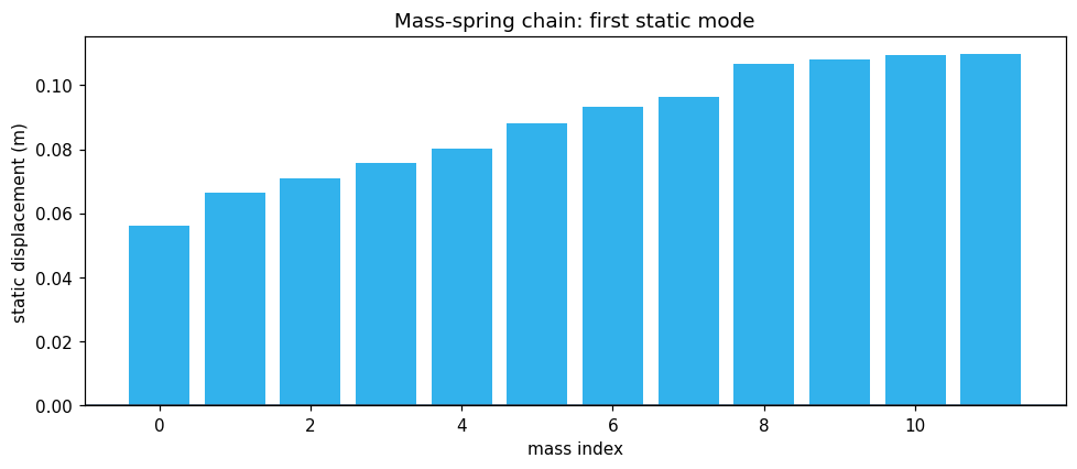
| Vibration | static displacement | 0.92 | converged |
| Heat exchanger | temperature field | 0.90 | converged |
| Truss | joint displacement | 0.77 | partial (12 epochs) |
| Molecular | total energy (log) | 0.51 | ranking ρ = 0.56 |
| Circuit | bus angle (DC power flow) | — | generator fixed, queued |
| Pipe flow | junction pressure | — | queued |
| Acoustic | wave field | — | queued |
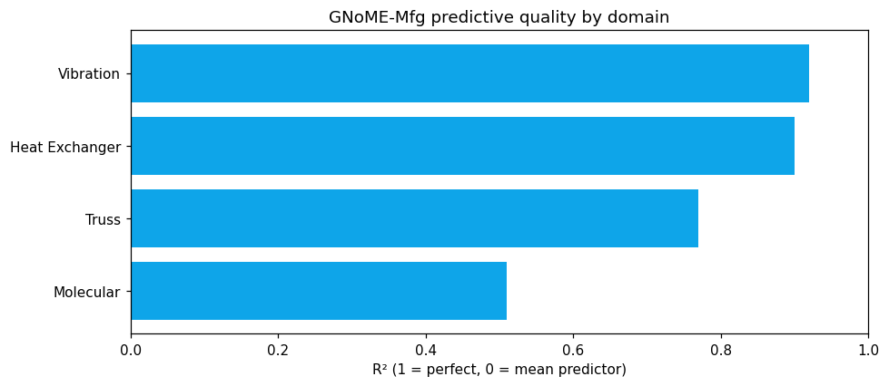
Four of seven domains beat the mean predictor with real margins. The queued rows are not idle: circuit previously failed because its flow target was random noise rather than a solved DC power flow. Acoustic failed because the model predicted acceleration while the rollout expected an increment. Both generators are now fixed and the full seven-domain run is queued on Kaggle GPU.
What we fixed to make this real
Silent failures are worse than loud failures. These five bugs each made a model silently worse than predicting the average.
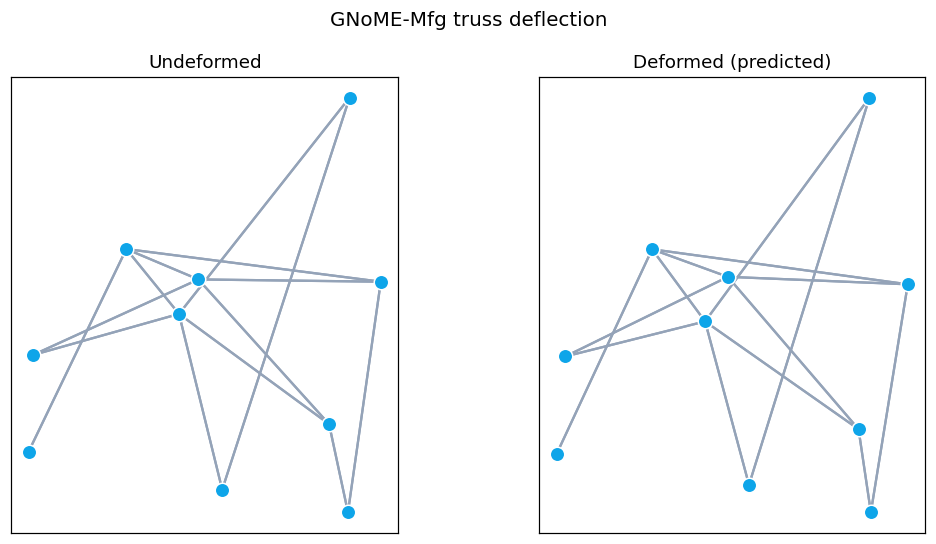
1. Truss readout ignored vector nature of displacement. The original readout predicted displacement from rotation-invariant scalars only. Displacement is a vector — when the truss rotates, its deflection field rotates with it. A readout that sees only scalars cannot represent this. Fix: scalar-gated equivariant readout that takes vector channels. R² went from −0.07 (worse than mean) to 0.77.
2. Circuit targets were random noise. The original circuit generator produced flow targets as random angles — not a real DC power flow solution. The model could not learn what was not a function. Fix: replaced with an exact DC power flow solve (B·θ = P with pseudo-inverse for islanded buses). Flow is now a real function of network topology.
3. Truss generator emitted isolated nodes with infinite deflection. With 40% edge retention probability, some nodes become isolated — zero incident stiffness → disp = loads × 0.05/1e-6 = 50,000 m. A single pathological graph corrupted the z-scalers for the entire dataset (sd = 4,336 instead of ~1). Fix: floor stiffness denominator at 0.01. R² went from −∞ (divergent) to 0.77.
4. Acoustic solver violated the CFL stability bound. The finite-difference time-domain (FDTD) solver used dt = 0.001 s with dx = 0.125 m and c = 343 m/s. CFL number = 343 × 0.001 / 0.125 = 2.74, exceeding the stability limit of ~0.7. The wave field diverged to NaN. Fix: dt = dx / (c × √3) ≈ 0.0002 s.
5. Physics loss compared incompatible units. The original physics term equated force and strain — different physical quantities with different scales. On z-scored targets this meant the physics loss was fighting the data loss on different manifolds. Fix: dual z-scored targets with Hooke's law as an evaluation metric, not a training loss.
Physics grounding
Each domain carries a differentiable physics residual used as an evaluation metric, not just a training loss:
| Domain | Governing law | How it's checked |
|---|---|---|
| Truss | Hooke's law (F = EA · ΔL/L) | Member stress vs strain on held-out loads |
| Circuit | DC power flow (B·θ = P) | Residual of the linear system |
| Acoustic | Wave equation (∂²p/∂t² = c²∇²p) | FDTD rollout vs predicted field |
| Heat | Fourier's law (q = −k∇T) | Temperature gradient consistency |
| Vibration | Static equilibrium (Ku = f) | Stiffness matrix residual |
| Molecular | Total energy decomposition | Energy prediction vs reference |
| Pipe | Darcy-Weisbach (ΔP = fL/D · ρv²/2) | Pressure drop vs flow rate |
The claim is not that we beat a finite-element solver. The claim is that the learned model and the governing law stay consistent on held-out data.
Simulation clips
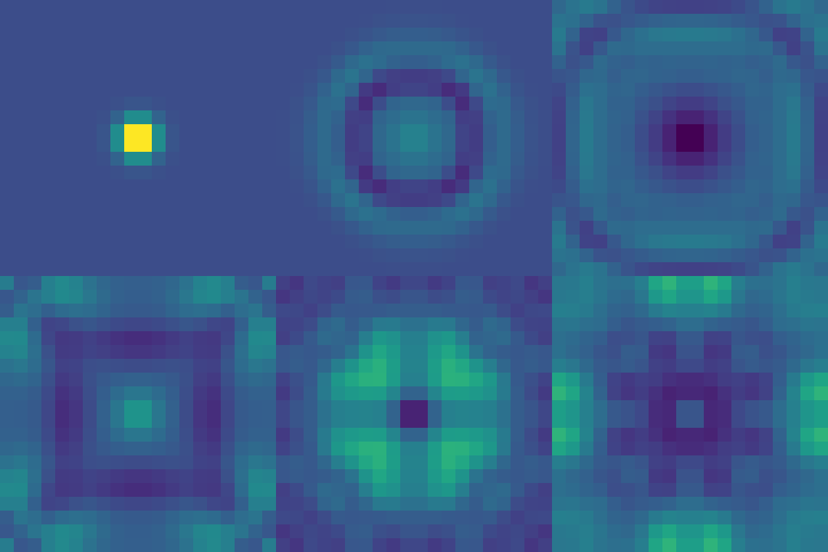
Limitations
What still falls short. (1) The datasets are synthetic. Truss and circuit generators use closed-form or linear-system solutions, not full finite-element or power-flow solvers. Real design data is the next input. (2) Two domains (circuit, acoustic) have not yet produced converged numbers under the corrected generators. We do not claim results we have not measured. (3) Three-layer message passing is shallow relative to long-range interactions in real engineering systems. Hierarchical multi-scale aggregation is implemented but not yet benchmarked. (4) The full seven-domain GPU run is queued. The verified numbers here come from local partial runs while that queue clears. (5) No real-world validation — every result is on synthetic data. The gap between synthetic and real is the gap between a paper and a product.
References
- Belbute-Peres et al., "Combining Differentiable PDE Solvers and Graph Neural Networks for Fluid Flow Prediction," 2020. arXiv
- Moseley et al., "Solving the wave equation with physics-informed deep learning," 2020. arXiv
- Raissi et al., "Physics-informed neural networks," Journal of Computational Physics, 2019. arXiv
- Sanchez-Gonzalez et al., "Learning to simulate complex physics with graph networks," ICML 2020. arXiv
- Merchant et al., "Scaling deep learning for materials discovery" (GNoME), Nature 2023. Nature
Code: github.com/sehajr-singhs/gnome-manufacturing · Related: GNOmE · PSN-1 · Showcase